华东理工大学2010—2011 学年 第 一 学期
《 应用统计学 》实验报告
班级 学号 姓名
开课学院 商学院 任课教师 成绩
实验报告:
4.1
―Analyze--Correlate --Bivariate‖
第一小题:
1
得到output如下

分析:Pearson相关系数为-0.744,P=0,应拒绝总体中这两个变量相关系数为零的假设。因此可认为,consump和income呈现出显著的负相关。
第二小题:
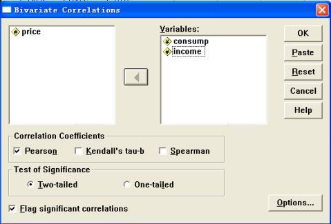
2
Ok后,得output,如下图
分析:我选取current salary和educational level这两个随机变量做相关分析。Pearson相关系数为0.661,P=0,应拒绝总体中这两个变量相关系数为零的假设。因此可认为,current salary和educational level呈现出显著的正相关。
4.2
―Analyze –Regression—Liner‖
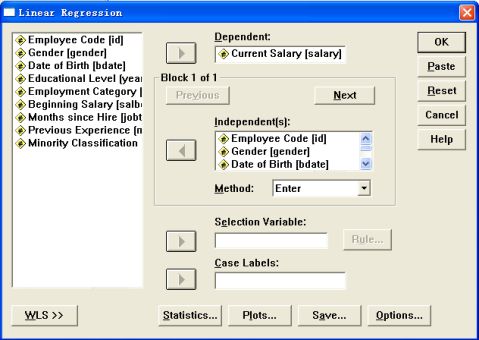
3
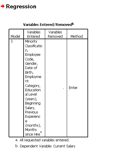
Method框选用Enter,得到output,如下图 表1:
4
表2:
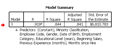
表3:
5
表4:

分析:表1,引入或剔除的变量;用强迫引入法。
表2,模型摘要;相关系数(R)=0.919、判定系数=0.844、调整判定系数=0.841、估计值的标准误=6810.783。 表3,方差分析;回归的均方=1.2E+11、剩余的均方=2.1E+11、F=278.909、P=0。可认为整个方程具有显著性。
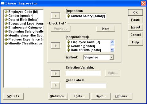
表4,回归分析中的系数;常数项=-15103.8,各个随机变量的回归系数、回归系数的标准误、标准化回归系数、回归系数t检验的t值、P值列表。可知只有Educational Level、Employment Category、Beginning Salary、Previous Experience这几个随机变量是与因变量是显著相关的,可知使用Enter方法有些系数是不显著的,下面使用Stepwise方法。

6
7 Variables Entered/Removed(a)
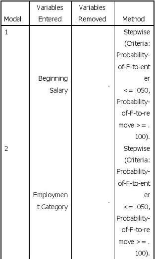
3 Stepwise
(Criteria:
Probability-
Previous of-F-to-ent
Experience . er (months) <= .050,
Probability-
of-F-to-re
move >= .
100).
4 Stepwise
(Criteria:
Probability-
of-F-to-ent
Employee
Code . er
<= .050,
Probability-
of-F-to-re
move >= .
100).
5 Stepwise
(Criteria:
Probability-
Educational of-F-to-ent
Level . er
(years) <= .050,
Probability-
of-F-to-re
move >= .
100).
6 Stepwise
(Criteria:
Probability-
of-F-to-ent
Gender . er
<= .050,
Probability-
of-F-to-re
move >= .
100).
a Dependent Variable: Current Salary
8
Model Summary
Adjusted R
Model 1 2 3 4 5 6
R .880(a) .898(b) .909(c) .915(d) .917(e) .918(f)
R Square
.775 .806 .827 .836 .841 .843
Square
.774 .805 .826 .835 .839 .841
Std. Error of the Estimate $8,119.791 $7,548.006 $7,133.578 $6,942.927 $6,860.175 $6,813.675
a Predictors: (Constant), Beginning Salary
b Predictors: (Constant), Beginning Salary, Employment Category
c Predictors: (Constant), Beginning Salary, Employment Category, Previous Experience (months)
d Predictors: (Constant), Beginning Salary, Employment Category, Previous Experience (months), Employee Code e Predictors: (Constant), Beginning Salary, Employment Category, Previous Experience (months), Employee Code, Educational Level (years)
f Predictors: (Constant), Beginning Salary, Employment Category, Previous Experience (months), Employee Code, Educational Level (years), Gender
Sum of
Model 1
Regression Residual Total
2
Regression Residual Total
3
Regression Residual Total
4
Regression Residual Total
Squares 106862706669.340 310535068
13.535 137916213482.875 111139190822.232 267770226
60.643 137916213482.875 114049771385.160 238664420
97.715 137916213482.875 115356631081.102 225595824
01.773 137916213
df
1
Mean Square 10686270666
9.340
F 1620.826
975.378
747.065
598.270
Sig. .000(a)
.000(b)
.000(c)
.000(d)
ANOVA(g)
471 65931012.343 472 2
55569595411.
116
470 56972388.640 472 3
38016590461.
720
469 50887936.242 472 4
28839157770.
275
468 48204235.901 472
9
482.875
5
Regression Residual Total
6
Regression Residual Total
115938259893.026 219779535
89.850 137916213482.875 116281618026.170 216345954
56.705 137916213482.875
a Predictors: (Constant), Beginning Salary
b Predictors: (Constant), Beginning Salary, Employment Category
c Predictors: (Constant), Beginning Salary, Employment Category, Previous Experience (months)
d Predictors: (Constant), Beginning Salary, Employment Category, Previous Experience (months), Employee Code e Predictors: (Constant), Beginning Salary, Employment Category, Previous Experience (months), Employee Code, Educational Level (years)
f Predictors: (Constant), Beginning Salary, Employment Category, Previous Experience (months), Employee Code, Educational Level (years), Gender g Dependent Variable: Current Salary
Unstandardized Coefficients
Model 1 2
(Constant) Beginning Salary (Constant) Beginning Salary Employment Category
3
(Constant) Beginning Salary Employment Category Previous Experience (months)
4
(Constant) Beginning Salary Employment Category
5918.889
1.476 6061.775
979.032
.062 631.157
.680 .274
6.046 23.831 9.604
.000 .000 .000
-23.768
3.143
-.146
-7.563
.000
B 1929.517
1.910 1038.773
1.469 5937.464 3043.572
1.468 6146.203
Std. Error 889.168
.047 832.923
.067 685.314 830.627
.064 648.274
Standardized Coefficients
Beta
.880
.677 .269
.677 .278
t 2.170 40.259 1.247 21.829 8.664 3.664 23.080 9.481
Sig. .031 .000 .213 .000 .000 .000 .000 .000
Coefficients(a) 5
23187651978.
605
492.704
417.443
.000(e)
.000(f)
467 47061999.122 472 6
19380269671.
028
466 46426170.508 472
10
Previous Experience (months) Employee Code
5
(Constant) Beginning Salary Employment Category Previous Experience (months) Employee Code Educational Level (years)
6
(Constant) Beginning Salary Employment Category Previous Experience (months) Employee Code Educational Level (years) Gender
a Dependent Variable: Current Salary
Collinearity
Partial
Model 1
Employee Code Gender Date of Birth Educational Level (years) Employment Category Months since Hire Previous Experience (months) Minority
-.040(a)
-1.809 11
.071
-.083
.975
-.138(a)
-6.571
.000
-.290
.998
Beta In -.102(a) -.061(a) .136(a) .173(a) .269(a) .101(a)
t -4.754 -2.509 6.471 6.385 8.664 4.707
Sig. .000 .012 .000 .000 .000 .000
Correlation
-.214 -.115 .286 .283 .371 .212
Statistics Tolerance
1.000 .792 1.000 .599 .429 1.000
Excluded Variables(g) -10.929 471.942 -1984.915
2.310 153.876 729.877
-.087 .080 -.058
-4.732 3.067 -2.720
.000 .002 .007
-21.447
3.302
-.131
-6.495
.000
-11.449 537.847 2845.794
1.327 5795.143
2.318 152.993 2082.933
.070 622.529
-.092 .091
.612 .262
-4.940 3.516 1.366 19.007 9.309
.000 .000 .173 .000 .000
-19.577
3.251
-.120
-6.021
.000
-12.166 288.011 1.364 5856.232
2.337 1871.181
.069 626.369
-.097
.629 .265
-5.207 .154 19.764 9.349
.000 .878 .000 .000
-23.791
3.059
-.146
-7.778
.000
Classification
2
Employee Code Gender Date of Birth Educational Level (years) Months since Hire Previous Experience (months) Minority Classification
3
Employee Code Gender Date of Birth Educational Level (years) Months since Hire Minority Classification
4
Gender Date of Birth Educational Level (years) Months since Hire Minority Classification
5
Gender Date of Birth Months since Hire Minority Classification
6
Date of Birth Months since Hire Minority Classification
-.033(b) -.097(c) -.078(c) .067(c) .102(c) .096(c) -.010(c) -.068(d) .081(d) .091(d) -.280(d) -.013(d) -.058(e) .069(e) -.225(e) -.015(e) .047(f) -.111(f) -.023(f)
-1.601 -5.207 -3.614 2.068 3.870 5.142 -.521 -3.214 2.595 3.516 -.883 -.699 -2.720 2.201 -.718 -.765 1.434 -.354 -1.185
.110 .000 .000 .039 .000 .000 .602 .001 .010 .000 .378 .485 .007 .028 .473 .445 .152 .723 .237
-.074 -.234 -.165 .095 .176 .231 -.024 -.147 .119 .161 -.041 -.032 -.125 .101 -.033 -.035 .066 -.016 -.055
.974 .999 .769 .354 .516 .999 .950 .761 .352 .512 .003 .949 .743 .346 .003 .949 .313 .003 .928
-.146(b)
-7.563
.000
-.330
.996
-.097(b) -.050(b) .140(b) .157(b) .096(b)
-4.894 -2.186 7.273 6.212 4.834
.000 .029 .000 .000 .000
-.220 -.100 .318 .276 .218
.999 .789 .999 .596 .999
a Predictors in the Model: (Constant), Beginning Salary
b Predictors in the Model: (Constant), Beginning Salary, Employment Category
c Predictors in the Model: (Constant), Beginning Salary, Employment Category, Previous Experience (months) d Predictors in the Model: (Constant), Beginning Salary, Employment Category, Previous Experience (months), Employee Code
12
e Predictors in the Model: (Constant), Beginning Salary, Employment Category, Previous Experience (months), Employee Code, Educational Level (years)
f Predictors in the Model: (Constant), Beginning Salary, Employment Category, Previous Experience (months), Employee Code, Educational Level (years), Gender
g Dependent Variable: Current Salary
上面是使用Stepwise方法得出的output,除了Constant之外都显著。
结论:由倒数第二张表格可知,使用Stepwise方法得到的不显著的值比Enter方法少,使用Stepwise方法比Enter方法好。
13