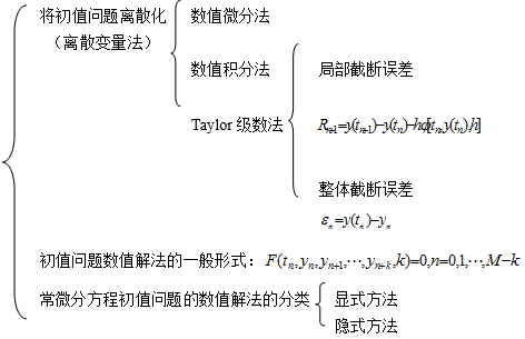
第7章 常微分方程初值问题的数值解法
--------学习小结
一、 本章学习体会
本章的主要内容是要掌握如何用数值解代替其精确解,这对于一些特殊的微分方程,特别是一些不好解其通解方程是非常有用的。对于本章我总结如下几点:
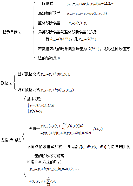
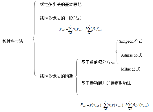
1、本章计算量相对较小,重要是其思想。在做题过程中,要理解各种方法的原理及推导过程。
2、本章对泰勒展开法有一定要求。无论是求方法的阶数还是推导数值解法的公式经常用到泰勒展开。因此,我们对于泰勒级数要有很清楚的认识。
3、在求数值解法的公式推导时,经常用到第六章的插值型求积公式。可见,在整本书中,知识往往是贯通的。
二、 本章知识梳理
相容性,收敛性和绝对稳定性
1、相容性:
设增量函数 在区域
在区域 上连续,且对
 满足Lipschitz条件,则单步法与微分方程相容的充要条件是单步法至少是一阶的方法
2、收敛性;
(1)定义:若对任意的 及任意的
及任意的 ,极限
,极限 则称单步法是收敛的
(2)单步法的收敛的充要条件:
(3)收敛与相容的关系:
设增量函数在区域上连续,且对 满足Lipschitz条件,则单步法与微分方程相容的充要条件是单步法是收敛的
3、稳定性(描述初始值的误差对计算结果的影响)
4、绝对稳定性:
三、 本章思考题
试用数值积分法建立常微分方程的初值问题:
 的数值求解公式:
解:由 得:
得: (1)
(1)
对于(1)式。左右两边同时在 上积分得:
上积分得:

左边= (2)
(2)
右边= (3)
(3)
其中
带入(3)式化简整理可得:

将(2)(3)带入(1)中可得:
四、 本章检测题
试用Taylor级数法(取p=2)导出求解初值问题
 的数值方法,并指出此方法的阶。
解: 


令t=tn, ,
,
则  , n=0,1,2…
由于  ,所以此方法为二阶方法。
第二篇:数值分析的一个小结
InterpolationandPolynomialApproximation
XueJingnan(200805090173)
April1,2011
Abstract
Inthisreport,wereviewedthreedi?erentinterpolationsandpolynomialap-proximations[1]respectively,say,LagrangePolynomial,HermiteInterpolationandCubicSplineInterpolation.Weintroducedtheiralgorithmdescriptions,relatedmathematicaldeductionsandapplicationstopracticalproblemsrespec-tively.Moreover,abriefdiscussionoftheiradvantagesandlimitsarepresentedatlast.
Contents
1Introduction
2InterpolationandtheLagrangePolynomial
2.1Mathematicaldeduction.......................
2.2Numericalexperiments........................
2.2.1Example1...........................
2.2.2Example2...........................3HermiteInterpolation
3.1Mathematicaldeduction.......................
3.2Algorithmdescription........................
3.2.1pseudocode..........................
3.2.2code..............................
3.3Numericalexperiments........................
3.3.1Example1...........................
3.3.2Example2...........................4CubicSplineInterpolation
4.1Mathematicaldeduction.......................
4.2Algorithmdescription........................
4.2.1pseudocode..........................
4.2.2code..............................
4.3Numericalexperiments........................
4.3.1Example1...........................
4.3.2Example2...........................5DiscussionandConclusion
5.1InterpolationandtheLagrangePolynomial............
5.2HermiteInterpolation........................
5.3CubicSplineInterpolation......................
124xxxxxxxxxxxx21213161xxxxxxxxxxxx23232323
Chapter1
Introduction
Oneofthemostusefulandwell-knownclassesoffunctionsmappingthesetofrealnumbersintoitselfistheclassofalgebraicpolynomials,thesetoffunctionsoftheform
Pn(x)=anxn+an?1xn?1+···+a1x+a0
wherenisanonnegativeintegeranda0,...,anarerealconstants.Onereasonfortheirimportanceisthattheyuniformlyapproximatecontinuousfunctions.Givenanyfunction,de?nedandcontinuousonaclosedandboundedinter-val,thereexistsapolynomialthatisas”close”tothegivenfunctionasdesired.Anotherimportantreasonforconsideringtheclassofpolynomialsintheapprox-imationoffunctionsisthatthederivativeandinde?niteintegralofapolynomialareeasytodetermineandarealsopolynomials.Forthesereasons,polynomialsareoftenusedforapproximatingcontinuousfunctions.
Inthisreport,wediscussedapproximatingafunctionusingpolynomialsandpiecewisepolynomials.Thefunctioncanbespeci?edbyagivende?ningequationorbyprovidingpointsintheplanethroughwhichthegraphofthefunctionpasses.Asetofnodesx0,x1,···,xnisgivenineachcase,andmoreinformation,suchasthevalueofvariousderivatives,mayalsoberequired.Weneedto?ndanapproximatingfunctionthatsatis?estheconditionsspeci?edbythesedata
TheinterpolatingpolynomialP(x)isthepolynomialofleastdegreethatsatis?es,forafunctionf,
P(xi)=f(xi),foreachi=0,1,...,n.
Althoughthisinterpolatingpolynomialisunique,itcantakemanydi?erentforms.TheLagrangeformismostoftenusedforinterpolatingtableswhennissmallandforderivingformulasforapproximatingderivativesandintegrals.Neville’smethodisusedforevaluatingseveralinterpolatingpolynomialsforcomputationandarealsousedextensivelyforderivingformulasforsolvingdi?erentialequations.TheHermitepolynomialsinterpolateafunctionandits
2
CHAPTER1.INTRODUCTION3derivativeatthenodes.Theycanbeveryaccuratebutrequiremoreinformationaboutthefunctionbeingapproximated.Whentherearealargenumberofnodes,theHermitepolynomialsalsoexhibitoscillationweaknesses.
However,polynomialinterpolationhastheinherentweaknessesofoscillation,particularlyifthenumberofnodesislarge.Inthiscase,thereareothermethodsthatcanbebetterapplied,themostcommonlyusedoneofwhichispiecewise-polynomialinterpolation.Iffunctionandderivativevaluesareavailable,piece-wisecubicHermiteinterpolationisrecommended.Thisisthepreferredmethodforinterpolatingvaluesoffunctionthatisthesolutiontoadi?erentequation.Whenonlythefunctionvaluesareavailable,freecubicsplineinterpolationcanbeused.Thissplineforcesthesecondderivativeofthesplinetobezeroattheendpoints.Othercubicsplinesrequireadditionaldata.Forexample,theclampedcubicsplineneedsvaluesofthederivativeofthefunctionattheend-pointsoftheinterval.
Chapter2
InterpolationandtheLagrangePolynomial
2.1Mathematicaldeduction
Theproblemofdeterminingapolynomialofdegreeonethatpassesthroughthedistinctpoints(x0,y0)and(x1,y1)isthesameasapproximatingafunctionfforwhichf(x0)=y0andy(x1)=y1bymeansofa?rst-degreepolynomialinterpolating,oragreeingwith,oragreeingwith,thevaluesoffatthegivenpoints.We?rstde?nethefunctions
L0(x)=
andthende?ne
P(x)=L0(x)f(x0)+L1(x)f(x1).
Since
L0(x0)=1,L0(x1)=0,L1(x0)=0,
wehave
P(x0)=1·f(x0)+0·f(x1)=f(x0)=y0
and
P(x1)=0·f(x0)+1·f(x1)=f(x1)=y1
SoPistheuniquelinearfunctionpassingthrough(x0,y0)and(x1,y1).Togeneralizetheconceptoflinearinterpolation,considertheconstructionofapolynomialofdegreeatmostnthatpassesthroughthen+1points
(x0,f(x0),(x1,f(x1),...(xn,f(xn).
Inthiscaseweneedtoconstruct,foreachk=0,1,...,n,afunctionLn,k(x)withthepropertythatLn,k(xi)=0wheni=kandLn,k(xk)=1.Tosatisfy
4andL1(x1)=1,x?x1x0?x1andL1(x)=x?x0x1?x0
CHAPTER2.INTERPOLATIONANDTHELAGRANGEPOLYNOMIAL5Ln,k(xi)=0foreachi=krequiresthatthenumeratorofLn,k(x)containstheterm
(x?x0)(x?x1)(x?x2)···(x?xk?1)(x?xk+1)···(x?xn).
TosatisfyLn,k(x)=1,thedenominatorofLn,k(x)mustbeequaltothistermevaluatedatx=xk.Thus,
Ln,k(x)=(x?x0)(x?x1)(x?x2)···(x?xk?1)(x?xk+1)···(x?xn).(xk?x0)(xk?x1)(xk?x2)···(xk?xk?1)(xk?xk+1)···(xk?xn)
TheinterpolatingpolynomialiseasilydescribedoncetheformofLn,kisknown.Thispolynomial,calledthenthLagrangeinterpolatingpolyno-mial,isde?nedinthefollowingtheorem.
Theorem2.1Ifx0,x1,···,xnaren+1distinctnumbersandfisafunctionwhosevaluesaregivenatthesenumbers,thenauniquepolynomialP(x)ofdegreeatmostnexistswith
f(xk)=P(xk),
Thispolynomialisgivenby
P(x)=f(x0)Ln,0(x)+···+f(xn)Ln,n(x)=
where,foreachk=0,1,···,n,
Ln,k(x)=(x?x0)(x?x1)(x?x2)···(x?xk?1)(x?xk+1)···(x?xn)
(xk?x0)(xk?x1)(xk?x2)···(xk?xk?1)(xk?xk+1)···(xk?xn)n?x?xi.=x?xkii=0i=kn?k=0foreachk=0,1,...,n.f(xk)Ln,k(x),(2.1)
(2.2)
WewillwriteLn,k(x)simplyasLk(x)whenthereisnoconfusionastoitsdegree
2.2
2.2.1NumericalexperimentsExample1
Usingthenumbers(ornodes)x0=2,x1=2.5,andx2=4to?ndthesecondin-terpolatingpolynomialforf(x)=1/xrequiresthatwedeterminethecoe?cientpolynomialsL0(x),L1(x),andL2(x).Innestedformtheyare
(x?2.5)(x?4)=(x?6.5)x+10,(2?2.5)(2?4)
(?4x+24)x?32(x?2)(x?4)L1(x)==,(2.5?2)(2.5?4)3L0(x)=
CHAPTER2.INTERPOLATIONANDTHELAGRANGEPOLYNOMIAL6and
L2(x)=(x?2)(x?2.5)(x?4.5)x+5=(4?2)(4?2.5)3
Sincef(x0)=f(2)=0.5,f(x1)=f(2.5)=0.4,andf(x2)=f(4)=0.25,wehave
P(x)=2?
k=0f(xk)Lk(x)
(x?4.5)x+5(?4x+24)x?32)+0.2533=0.5((x?6.5)x+10)+0.4(
=(0.05x?0.425)x+1.15.
Anapproximationtof(3)=1/3is
f(3)≈P(3)=0.325
2.2.2Example2
Forthegivenfunctionsf(x),letx0=0,x1=0.6,andx2=0.9.Constructinterpolationpolynomialsofdegreeatmosttwotoapproximatef(0.45),and?ndtheactualerror.
(1)
(2)
(3)
(4)f(x)=cosx√f(x)=f(x)=ln(x+1)f(x)=tanx
Atthebeginning,wedeterminedthecoe?cientpolynomialsL0(x),L1(x),andL2(x).Innestedformtheyare
50(x?0.6)(x?0.9)=[(x?1.5)x+0.54]+10,(0?0.6)(0?0.9)27
(x?0)(x?0.9)50L1(x)==?(x?0.9)x)(0.6?0)(0.6?0.9)9
(x?0)(x?0.6)100L2(x)==(x?0.6)x(0.9?0)(0.9?0.6)27L0(x)=
(1)f(x)=cosx
Sincef(x0)=f(0)=1,f(x1)=f(0.6)=cos(0.6)≈0.8253,
andf(x2)=f(0.9)≈0.6216,wehave
P(x)=2?
k=0f(xk)Lk(x)
≈(5010050[(x?1.5)x+0.54]+0.8253[?(x?0.9)x)]+0.6216[(x?0.6)x]27927
≈(?0.4309x?0.0326)x+1
CHAPTER2.INTERPOLATIONANDTHELAGRANGEPOLYNOMIAL7
Anapproximationtof(0.45)=cos(0.45)=0.9004is
f(0.45)≈P(0.45)=0.8980
Andtheactualerrorisf(0.45)?P(0.45)=2.4×10?3
√(2)f(x)=Sincef(x0)=f(0)=1,f(x1)=f(0.6)≈1.2649,
andf(x2)=f(0.9)≈1.3784,wehave
P(x)=2?
k=0f(xk)Lk(x)
≈(5010050[(x?1.5)x+0.54]+1.2649[?(x?0.9)x)]+1.3784[(x?0.6)x]≈(?0.0702x+0.4836)x+1
Anapproximationtof(0.45)=1.2042is
f(0.45)≈P(0.45)=1.2034
Andtheactualerrorisf(0.45)?P(0.45)=7.955×10?4
(3)f(x)=ln(1+x)
Sincef(x0)=f(0)=0,f(x1)=f(0.6)≈0.4700,
andf(x2)=f(0.9)≈0.6419,wehave
P(x)=2?
k=0f(xk)Lk(x)
≈0.4700[?10050(x?0.9)x)]+0.6419[(x?0.6)x]927
≈(?0.2337x+0.9236)x
Anapproximationtof(0.45)=0.3716is
f(0.45)≈P(0.45)=0.3683
Andtheactualerrorisf(0.45)?P(0.45)=3.3×10?3
(4)f(x)=tanx
Sincef(x0)=f(0)=0,f(x1)=f(0.6)≈0.6841,
andf(x2)=f(0.9)≈1.2602,wehave
P(x)=2?
k=0f(xk)Lk(x)
≈0.6841[?10050(x?0.9)x)]+1.2602[(x?0.6)x]927
≈(0.8669x+0.6200)x
CHAPTER2.INTERPOLATIONANDTHELAGRANGEPOLYNOMIAL8
Anapproximationtof(0.45)=0.4830is
f(0.45)≈P(0.45)=0.4545
Andtheactualerrorisf(0.45)?P(0.45)=0.0285
Chapter3
HermiteInterpolationLetx0,x1,...,xnben+1distinctnumbersin[a,b]andmibeanonnegativeintegerassociatedwithxi,fori=0,1,...,n.Supposethatf∈Cm[a,b],wherem=max0≤i≤nmi.TheosculatingpolynomialapproximatingfisthepolynomialP(x)ofleastdegreesuchthat
dkP(xi)dkf(xi)=,dxkdxkforeachi=0,1,...,nandk=0,1,...,nNotethatwhenn=0,theosculatingpolynomialapproximatingfisthem0thTaylorpolynomialforfatx0.Whenmi=0foreachi,theosculatingpolynomialisthenthLagrangepolynomialinterpolatingfonx0,x1,...,xnThecasewhenmi=1,foreachi,givestheHermitepolynomials.Foragivenfunctionf,thesepolynomialsagreewiththoseoff,theyhavethesame”shape”asthefunctionat(xi,f(xi))inthesensethatthetangentlinestothepolynomialandtothefunctionagree.Wewillrestrictourstudyofosculatingpolynomialstothissituation.
3.1Mathematicaldeduction
Firstly,consideratheoremthatdescribespreciselytheformoftheHermitepolynomials.
Theorem3.1Iff∈C1[a,b]andx0,...,xn∈[a,b]aredistinct,theuniquepolynomialofleastdegreeagreeingwithfandf?atx0,...,xnistheHermitepolynomialofdegreeatmost2n+1givenby
H2n+1(x)=
wheren?j=0f(xj)Hn,j(x)+n?j=0?n,j(x)f?(xj)H2Hn,j(x)=[1?2(x?xj)L?n,j(xj)]Ln,j(x)
9
CHAPTER3.HERMITEINTERPOLATION
and10?n,j(x)=(x?xj)L2Hn,j(x)
Inthiscontext,Ln,j(x)denotesthejthLagrangecoe?cientpolynomialofdegreende?nedinChapter2.
Moreover,iff∈C2n+2[a,b],then
(x?x0)2...(x?xn)22n+2f(ξ)f(x)=H2n+1(x)+(2n+2)!
forsomeξwitha<ξ<b
AlthoughTheorem3.1providesacompletedescriptionoftheHermitepoly-nomials,itisclearthattheneedtodetermineandevaluatetheLagrangepoly-nomialsandtheirderivativesmakestheproceduretediousevenforsmallvaluesofn.AnalternativemethodforgeneratingHermiteapproximationshasasitsbasistheNewtoninterpolatorydivided-di?erenceformulafortheLagrangepolynomialatx0,x1,...,xn,
Pn(x)=f[x0]+n?
k=1f[x0,x1,...,xk](x?x0)···(x?xk?1)
andtheconnectionbetweenthenthdivideddi?erenceandnthderivativeoff.
Supposethatthedistinctnumbersx0,x1,/dots,xnaregiventogetherwiththevaluesoffandf?atthesenumbers.De?neanewsequencez0,z1,...,z2n+1by
z2i=z2i+1=xi,foreachi=0,1,...,n,
andconstructthedivideddi?erencetablethatusesz0,z1,....z2n+1
Sincez2i=z2i+1=xi,foreachi,wecannotde?nef[z2i,z2i+1]bythedivideddi?erenceformula.Ifweassumethatthereasonablesubstitutioninthissituationisf[z2i,z2i+1]=f?(z2i)=f?(xi),wecanusetheentries
f?(x0),f?(x1),...,f?(xn)
inplaceoftheunde?ned?rstdivideddi?erences
f[z0,z1],f[z2,z3],...,f[z2n,z2n+1]
Theremainingdivideddi?erencesareproducedasusual,andtheappropriatedivideddi?erencesareemployedinNewton’sinterpolatorydivided-di?erenceformula.
TheHermitepolynomialisgivenby
H2n+1(x)=f[z0]+2n+1?
k=1f[z0,...,xk](x?z0)(x?z1)...(x?zk?1)
CHAPTER3.HERMITEINTERPOLATION11
3.2
3.2.1Algorithmdescriptionpseudocode
Toobtainthecoe?cientsoftheHermiteinterpolatingpolynomialH(x)onthe(n+1)distinctnumbersx0,...,xnforthefunctionf:
INPUTnumbersx0,x1,...,xn;valuesf(x0),...,f(xn)andf?(x0),...,f?(xn)OUTPUTthenumbersQ0,0,Q1,1,...,Q2n+1,2n+1where
H(x)=Q0,0+Q1,1(x?x0)+Q2,2(x?x0)2+Q3,3(x?x0)2(x?x1)
+Q4,4(x?x0)2(x?x1)2+···
+Q2n+1,2n+1(x?x0)2(x?x1)2···(x?xn?1)2(x?xn)
Step1Fori=0,1,...,ndoStep2and3
Step2Setz2i=xi;
z2i+1=xi;
Q2i,0=f(xi);
Q2i+1,0=f(xi)
Q2i+1,1=f?(xi)
Step3Ifi=0thenset
2i,1=2i,0?Q2i?1,0
z2i?z2i?1
Step4Fori=2,3,...,2n+1
forj=2,3,...,iset
QQQ
i,j=i,j?1?i?1,j?1
zi?zi?j
Step5OUTPUT(Q0,0,Q1,1...Q2n+1,2n+1)
STOP
CHAPTER3.HERMITEINTERPOLATION12
3.2.2code
3.3
3.3.1NumericalexperimentsExample1
UsetheHermitepolynomialthatagreeswiththedatainTable3.1to?ndanapproximationoff(1.5)
Table3.1:Example1
k
2
3xk1.61.9f(xk)0.45540220.2818186f?(xk)?0.5698959?0.5811571
Table3.2showstheentriesthatareusedfordeterminingtheHermitepoly-nomialH5(x)forx0,x1,andx2.
TheentriesinTable3.3usethegivendata.
CHAPTER3.HERMITEINTERPOLATION13H5(1.5)=0.6200860+(1.5?1.3)(?0.5220232)+(1.5?1.3)2(?0.0897427)
+(1.5?1.3)2(1.5?1.6)(0.0663657)+(1.5?1.3)2(1.5?1.6)2(0.0026663)+(1.5?1.3)2(1.5?1.6)2(1.5?1.9)(?0.0027738)
=0.5118277
3.3.2Example2
UseHermiteinterpolationtoconstructanapproximatingpolynomialforthefollowingdataTheentriesinTable3.5usethegivendata.
H5(x)=?0.0247500+(x+0.5)(0.7510000)+(x+0.5)2(2.7510000)+(x+0.5)2(x+0.25)
CHAPTER3.HERMITEINTERPOLATION14
Table3.2:
00z1=x0z2=x1z3=x1z4=x2z5=x2
00f[z1]=f(x0)
f[z1,z2]=
f[z2]=f(x1)f[z3]=f(x1)
f[z3,z4]=
f[z4]=f(x2)f[z5]=f(x2)
f[z0,z1]=f?(x0)
f[z2]?f[z1]21?
di?erences
f[z0,z1,z2]f[z1,z2,z3]f[z2,z3,z4]f[z3,z4,z5]
f[z2,z3]=f(x1)
f[z4]?f[z3]43
f[z4,z5]=f?(x2)
di?erencesdi?erences
f[z0,z1,z2,z3]
f[z0,z1,z2,z3,z4]
f[z1,z2,z3,z4]
f[z1,z2,z3,z4,z5]
f[z2,z3,z4,z5]
f[z0,z1,z2,z3,z4,z5]
CHAPTER3.HERMITEINTERPOLATION15
Table3.3:
1.31.61.61.91.9
-0.5220232
0.6200860
-0.5489460
0.4554022
-0.5698959
0.4554022
-0.5786120
0.2818186
-0.5811571
0.2818186
-0.0084837-0.0290537
0.0685667
-0.0698330
0.0679655
0.0010020
-0.0897427
0.0663657
0.0026663
-0.0027738
Table3.4:Example2
k23
xk?0.250
f(xk)0.33493751.101000
f?(xk)2.18900004.0020000
Table3.5:
-0.5-0.25-0.2500
0.7510000
-0.0247500
1.4387500
0.3349375
2.1890000
0.3349375
3.0642500
1.1010000
4.0020000
1.1010000
3.75100003.5010000
1
3.0010000
1
2.7510000
1
Chapter4
CubicSplineInterpolationThepreviouschapterconcernedtheapproximationofarbitraryfunctionsonclosedintervalsbytheuseofpolynomials.However,theoscillatorynatureofhigh-degreepolynomialsandthepropertythata?uctuationoverasmallportionoftheintervalcaninducelarge?uctuationsovertheentireragerestrictstheiruse.
Analternativeapproachistodividetheintervalintoacollectionofsubin-tervalsandconstructa(generally)di?erentapproximatingpolynomialoneachsubinterval.Approximationbyfunctionsofthistypeiscalledpiecewise-polynomialapproximation
Themostcommonpiecewise-polynomialapproximationusescubicpolyno-mialsbetweeneachsuccessivepairofnodesandiscalledcubicsplinein-terpolation.Ageneralcubicpolynomialinvolvesfourconstants,sothereissu?cient?exibilityinthecubicsplineproceduretoensurethattheinterpolantisnotonlycontinuouslydi?erentiableontheinterval,butalsohasacontinuoussecondderivative.Theconstructionofthecubicsplinedoesnot,however,as-sumethatthederivativesoftheinterpolantagreewiththoseofthefunctionitisapproximating,evenatthenodes.
4.1Mathematicaldeduction
Givenafunctionfde?nedon[a,b]andasetofnodesa=x0<x1</cdots<xn=b,acubicsplineinterpolantSforfisafunctionthatsatis?esthefollowingconditions:
a.S(x)isacubicpolynomial,denotedSj(x),onthesubinterval[xj,xj+1]foreachj=0,1,...,n?1;
b.S(xj)=f(xj)foreachj=0,1,...,n;
c.Sj+1(xj+1)=Sj(xj+1)foreachj=0,1,...,n?2;
??d.Sj+1(xj+1)=Sj(xj+1)foreachj=0,1,...,n?2;
16
CHAPTER4.CUBICSPLINEINTERPOLATION
????e.Sj+1(xj+1)=Sj(xj+1)foreachj=0,1,...,n?2;17
f.Oneofthefollowingsetsofboundaryconditionsissatis?ed:
(1)S??(x0)=S??(xn)=0(freeornaturalboundary)
(2)S?(x0)=f?(x0)andS?(xn)=f?(xn(clampedboundary)
Althoughcubicsplinesarede?nedwithotherboundaryconditions,thecon-ditionsgivenin(f)aresu?cientforourpurposes.Whenthefreeboundaryconditionsoccur,thesplineiscalledanaturalspline,anditsgraphapproxi-matestheshapethatalong?exiblerodwouldassumeifforcedtogothroughthedatapoints{(x0,f(x0)),(x1,f(x1)),...,(xn,f(xn))}.Inthischapter,weonlyconsiderthisone
Toconstructthecubicsplineinterpolantforagivenfunctionf,thecondi-tionsinthede?nitionareappliedtothecubicpolynomials
Sj(x)=aj+bj(x?xj)+cj(x?xj)2+dj(x?xj)3
foreachj=0,1,...,n?1.
Since
Sj(xj)=aj=f(xj)
condition(c)canbeappliedtoobtain
aj+1=Sj+1(xj+1)=Sj(xj+1)=aj+bj(xj+1?xj)+cj(xj+1?xj)2+dj(xj+1?xj)3foreachj=0,1,...,n?2.
Sincethetermsxj+1?xjareusedrepeatedlyinthisdevelopment,itisconvenienttointroducethesimplernotation
hj=xj+1?xj
foreachj=0,1,...,n?1..Ifwealsode?nean=f(xn),thentheequation
3aj+1=aj+bjhj+cjh2j+djhj(4.1)
holdsforeachj=0,1,...,n?2
Inasimilarmanner,de?nebn=S?(xn)andobservethat
?Sj(x)=bj+2cj(x?xj)+3dj(x?xj)2
?impliesSj(xj)=bj,foreachj=0,1,...,n?1.Applyingcondition(d)gives
bj+1=bj+2cjhj+3djh2j,(4.2)
foreachj=0,1,...,n?2
Anotherrelationshipbetweenthecoe?cientsofSjisobtainedbyde?ningcn=S??(xn)/2andapplyingcondition(e).Then,foreachj=0,1,...,n?1,
cj+1=cj+3djhj(4.3)
CHAPTER4.CUBICSPLINEINTERPOLATION18
SolvingfordjinEq.(4.3)andsubstitutingthisvalueintoEqs.(4.1)and(4.2)gives,forj=0,1,...,n?1,thenewequations
aj+1
and
bj+1=bj+hj(cj+cj+1)(4.5)
The?nalrelationshipinvolvingthecoe?cientsisobtainedbysolvingtheappropriateequationintheformofequation(3.4),?rstforbj,
bj=hj1(aj+1?aj)?(2cj+cj+1)hj3(4.6)h2j=aj+bjhj+(2cj+cj+1)3(4.4)
andthen,withareductionoftheindex,forbj?1.Thisgives
bj?1=1
hj?1(aj?aj?1)?hj?1(2cj?1+cj),3
SubstitutingthesevaluesintotheequationderivedfromEq(4.5),withtheindexreducedbyone,givesthelinearsystemofequations.
hj?1cj?1+2(hj?1+hj)cj+hjcj+1=33(aj+1?aj)?(aj?aj?1)(4.7)hjhj?1
foreachj=1,2,...,n?1.Thissysteminvolvesonlythe{cj}nj=0asunknowns
n?1sincethevaluesof{hj}j=0and{aj}nj=0aregiven,respectively,bythespacing
nofthenodes{xj}j=0andthevaluesoffatthenodes.
Notethatoncethevaluesof{cj}nj=0aredetermined,itisasimplematterto
?1n?1?ndtheremainderoftheconstants{bj}nj=0fromEq.(4.6)and{dj}j=0from
?1Eq.(4.3),andtoconstructthecubicpolynomials{Sj(x)}nj=0.
Themajorquestionthatarisesinconnectionwiththisconstructioniswhetherthevaluesof{cj}nj=0canbefoundusingthesystemofequationsgiveninEq.(4.7)and,ifso,whetherthesevaluesareunique.Thefollowingtheoremsindicatethatthisisthecasewhenthefreeornaturalboundaryisimposed.Astheproofofthistheoremrequiresomeknowledgewehaven’tlearned,wedecidenottointroducetheprooftothisreport.
Theorem4.1Iffisde?nedata=x0<x1<···<xn=b,thenfhasauniquenaturalsplineinterpolantSonthenodesx0,x1,....xn;thatis,asplineinterpolantthatsatis?estheboundaryconditionsS??(a)=0andS??(b)=0.
4.2
4.2.1Algorithmdescriptionpseudocode
ToconstructthecubicsplineinterpolantSforthefunctionf,de?nedatthenumbersx0<x1<···<xn,satisfyingS??(x0)=S??(xn)=0:
CHAPTER4.CUBICSPLINEINTERPOLATIONINPUTn;x0,x1,...,xn;a0=f(x0),a1=f(x1),...,an=f(xn).OUTPUTaj,bj,cj,djforj=0,1,...,n?1.Step1Fori=0,1,...,n?1sethi=xi+1?xi.Step2Fori=1,...,n?1set
αi=Step3Setl0=1;
u0=0;
z0=0;
Step4Fori=1,2,...,n?1
setli=2(xi+1?xi?1)?hi?1ui?1;
ui=hi/li
zi=(αi?hi?1zi?1)/li
Step5Setln=1;
zn=0;
cn=0;
Step6Forj=n?1,n?2,...,0
setcj=zj?ujcj+1;
bj=(aj+1?aj)/hj?hj(cj+1+2cj)/3;
dj=(cj+1?cj)/(3hj).
Step7OUTPUT(aj,bj,cj,djforj=0,1,...,n?1)
STOP33(ai+1?ai)?(ai?ai?1)hihi?119
CHAPTER4.CUBICSPLINEINTERPOLATION20
4.2.2code
CHAPTER4.CUBICSPLINEINTERPOLATION21
4.3
4.3.1
Numericalexperiments
Example1
Table4.1:Example1
f(x)2.251.32.31.52.251.851.952.11.42.60.92.70.72.40.62.150.52.050.42.10.25
Usingthecodesabovetogeneratethefreecubicsplineforthisdataproducesthecoe?cientsshowninTable4.2.
Table4.2:
123xxxxxxxxxxxx3141516171819
j1.31.92.12.63.03.94.44.75.06.07.08.09.210.511.311.12.012.613.0
j1.51.852.12.62.72.42.152.052.12.252.32.251.951.40.90.70.60.50.4
j0.421.091.290.59-0.02-0.5-0.48-0.070.260.080.01-0.14-0.34-0.53-0.73-0.49-0.14-0.18-0.39
j-0.301.41-0.37-1.04-0.50-0.030.081.27-0.16-0.03-0.04-0.11-0.05-0.10-0.150.94-0.060.00-0.54
j0.95-2.96-0.450.450.170.081.31-1.580.040.00-0.020.02-0.01-0.021.21-0.840.04-0.450.60
4.3.2Example2
Constructthefreecubicsplineforthefollowingdata.
CHAPTER4.CUBICSPLINEINTERPOLATION22
Table4.3:Example2
0.2
0.3
0.4-0.283986680.006600950.24842440
Usingthecodesabovetogeneratethefreecubicsplineforthisdataproducesthecoe?cientsshownbelow.
Table4.4:
1
2j0.20.3j-0.28400.0066j3.18522.6171j-2.6987-2.9826j-0.94639.9421
Sincethecoe?cientshavebeendetermined,thepolynomialwillalsobearrivedateasily.
Chapter5
DiscussionandConclusionInthischapter,wewillanalyzeadvantagesandlimitationsofeachmethodre-spectively.
5.1InterpolationandtheLagrangePolynomialAmongthesemethods,theLagrangepolynomialisconsideredthesimplestone,meaningthatitneedstheleastworkload.However,astheLagrangepolynomialonlyrequiresthatthevaluesoftheinterpolatingpolynomialarethesamewiththoseoforiginalfunctiononthegivennodes,thereforeitsaccuracyisrelativelow,comparedwithHermitepolynomial.Moreover,ithastheinherentweaknessofoscillation,whichlimitsitsapplicationtosituationwherethenumberofnodesislarge.
5.2HermiteInterpolation
ComparedwiththeLagrangePolynomial,Hermitepolynomialinterpolateafunctionanditsderivativeatthenodes,thusitcanbeexpectedtobemoreaccurate.However,italsomeansthatmoreinformationaboutthefunctionbeingappropriatedwillberequired,whichlimitsitsapplicationtosituationswherenotenoughinformationabouttheoriginalpolynomialcanbeprovided.Andwhentherearealargeofnumberofnodes,theHermitepolynomialalsoexhibitoscillationweaknesses.
5.3CubicSplineInterpolation
Themostobviousadvantageofthisinterpolationisthatitsuccessfullysolvedtheinherentproblem,oscillatorynatureofhigh-degreepolynomial,withintheHermiteInterpolationandtheLagrangeInterpolation.However,theworkloadofthisinterpolationissomewhatheavierthanothers.
23
Bibliography
[1]RichardL.BurdenandJ.DouglasFaires:NumericalAnalysis,chapter3
(2001)
24