大学物理实验课程设计实验报告
姓名:郑友行 学号:10211388 班级:309
重力加速度的测定
一、实验任务: 精确测定北京地区的重力加速度
二、实验要求: 测量结果的相对不确定度不超过5%
三、物理模型的建立及比较 初步确定有以下六种模型方案:
方法一、用打点计时器测量 所用仪器为:打点计时器、直尺、带钱夹的铁架台、纸带、夹子、重物、学生电源等. 利用自由落体原理使重物做自由落体运动.选择理想纸带,找出起始点0,数出时间为t的P点,用米尺测出OP的距离为h,其中t=0.02秒×两点间隔数.由公式h=gt2/2得g=2h/t2,将所测代入即可求得g.
方法二、用滴水法测重力加速度 调节水龙头阀门,使水滴按相等时间滴下,用秒表测出n个(n取50—100)水滴所用时间t,则每两水滴相隔时间为t′=t/n,用米尺测出水滴下落距离h,由公式h=gt′2/2可得g=2hn2/t2.
方法三、取半径为R的玻璃杯,内装适当的液体,固定在旋转台上.旋转台绕其对称轴以角速度ω匀速旋转,这时液体相对于玻璃杯的形状为旋转抛物面 重力加速度的计算公式推导如下: 取液面上任一液元A,它距转轴为x,质量为m,受重力mg、弹力N.由动力学知: Ncosα-mg=0(1) Nsinα=mω2x(2) 两式相比得tgα=ω2x/g,又tgα=dy/dx,∴dy=ω2xdx/g, ∴y/x=ω2x/2g.∴g=ω2x2/2y. .将某点对于对称轴和垂直于对称轴最低点的直角坐标系的坐标x、y测出,将转台转速ω代入即可求得g.
方法四、光电控制计时法 调节水龙头阀门,使水滴按相等时间滴下,用秒表测出n个(n取50—100)水滴所用时间t,则每两水滴相隔时间为t′=t/n,用米尺测出水滴下落距离h,由公式h=gt′2/2可得g=2hn2/t2.
方法五、用圆锥摆测量 所用仪器为:米尺、秒表、单摆. 使单摆的摆锤在水平面内作匀速圆周运动,用直尺测量出h(见图1),用秒表测出摆锥n转所用的时间t,则摆锥角速度ω=2πn/t 摆锥作匀速圆周运动的向心力F=mgtgθ,而tgθ=r/h所以mgtgθ=mω2r由以上几式得: g=4π2n2h/t2. 将所测的n、t、h代入即可求得g值.
方法六、单摆法测量重力加速度 在摆角很小时,摆动周期为: 则 通过对以上六种方法的比较,本想尝试利用光电控制计时法来测量,但因为实验室器材不全,故该方法无法进行;对其他几种方法反复比较,用单摆法测量重力加速度原理、方法都比较简单且最熟悉,仪器在实验室也很齐全,故利用该方法来测最为顺利,从而可以得到更为精确的值。
四、采用模型六利用单摆法测量重力加速度:
摘要: 重力加速度是物理学中一个重要参量。地球上各个地区重力加速度的数值,随该地区的地理纬度和相对海平面的高度而稍有差异。一般说,在赤道附近重力加速度值最小,越靠近南北两极,重力加速度的值越大,最大值与最小值之差约为1/300。研究重力加速度的分布情况,在地球物理学中具有重要意义。利用专门仪器,仔细测绘各地区重力加速度的分布情况,还可以对地下资源进行探测。 伽利略在比萨大教堂内观察一个圣灯的缓慢摆动,用他的脉搏跳动作为计时器计算圣灯摆动的时间,他发现连续摆动的圣灯,其每次摆动的时间间隔是相等的,与圣灯摆动的幅度无关,并进一步用实验证实了观察的结果,为单摆作为计时装置奠定了基础。这就是单摆的等时性原理。 应用单摆来测量重力加速度简单方便,因为单摆的振动周期是决定于振动系统本身的性质,即决定于重力加速度g和摆长L,只需要量出摆长,并测定摆动的周期,就可以算出g值。
实验器材: 单摆装置(自由落体测定仪),钢卷尺,游标卡尺、电脑通用计数器、光电门、单摆线。
实验原理: 单摆是由一根不能伸长的轻质细线和悬在此线下端体积很小的重球所构成。在摆长远大于球的直径,摆锥质量远大于线的质量的条件下,将悬挂的小球自平衡位置拉至一边(很小距离,摆角小于5°),然后释放,摆锥即在平衡位置左右作周期性的往返摆动。摆锥所受的力f是重力和绳子张力的合力,f指向平衡位置。当摆角很小时(θ<5°),圆弧可近似地看成直线,f也可近似地看作沿着这一直线。设摆长为L,小球位移为x,质量为m,则 sinθ= f=psinθ=-mg=-mx(2-1) 由f=ma,可知a=-x 式中负号表示f与位移x方向相反。 单摆在摆角很小时的运动,可近似为简谐振动,比较谐振动公式:a==-ω2x 可得ω= 于是得单摆运动周期为: T=2π/ω=2π(2-2) T2=L(2-3) 或g=4π2(2-4) 利用单摆实验测重力加速度时,一般采用某一个固定摆长L,在多次精密地测量出单摆的周期T后,代入(2-4)式,即可求得当地的重力加速度g。 由式(2-3)可知,T2和L之间具有线性关系,为其斜率,如对于各种不同的摆长测出各自对应的周期,则可利用T2—L图线的斜率求出重力加速度g。
试验条件及误差分析: 上述单摆测量g的方法依据的公式是(2-2)式,这个公式的成立是有条件的,否则将使测量产生如下系统误差:
1.单摆的摆动周期与摆角的关系,可通过测量θ<5°时两次不同摆角θ1、θ2的周期值进行比较。在本实验的测量精度范围内,验证出单摆的T与θ无关。 实际上,单摆的周期T随摆角θ增加而增加。
2.根据振动理论,周期不仅与摆长L有关,而且与摆动的角振幅有关,其公式为: T=T0[1+()2sin2+()2sin2+……] 式中T0为θ接近于0o时的周期,即T0=2π 2.悬线质量m0应远小于摆锥的质量m,摆锥的半径r应远小于摆长L,实际上任何一个单摆都不是理想的,由理论可以证明,此时考虑上述因素的影响。
3.如果考虑空气的浮力,则周期应为: 式中T0是同一单摆在真空中的摆动周期,ρ空气是空气的密度,ρ摆锥是摆锥的密度,由上式可知单摆周期并非与摆锥材料无关,当摆锥密度很小时影响较大。
4.忽略了空气的粘滞阻力及其他因素引起的摩擦力。实际上单摆摆动时,由于存在这些摩擦阻力,使单摆不是作简谐振动而是作阻尼振动,使周期增大。
上述四种因素带来的误差都是系统误差,均来自理论公式所要求的条件在实验中未能很好地满足,因此属于理论方法误差。此外,使用的仪器如千分尺、米尺也会带来仪器误差。
实验步骤:
1.仪器调整: 本实验是在自由落体测定仪上进行,故需要把自由落体测定仪的支柱调成铅直。调整方法是:安装好摆锤后,调节底座上的水平调节螺丝,使摆线与立柱平行。
2.测量摆长L 测量摆线支点与摆锥(因实验室无摆球,用摆锥代替)质心之间的距离L。由于摆锥质心位置难找,可用米尺测悬点到摆锥最低点的距离L1,(测六次),用千分尺测摆锥的直径d,(测六次),则摆长: L=L1-d/2 3.测量摆动周期T 使摆锥摆动幅度在允许范围内,
3.测量摆锥往返摆动50次所需时间t,重复测量6次,求出T=t/50。测量时,选择摆锥通过最低点时开始计时,最后计算时单位统一为秒。
4.将所测数据列于表中,并计算出摆长、周期及重力加速度。
5.实验数据处理 实验数据记录及处理
(1)试验数据记录 仪器误差限:游标卡尺Δm=0.02mm,米尺Δm=1mm,电脑通用计数器Δm=0.0001ms。
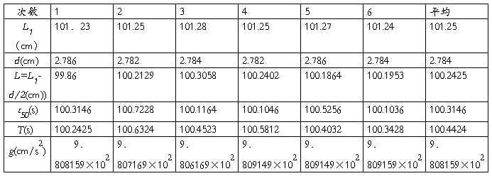
(2)实验数据处理: 重力加速度的最后结果为 g=(9.808159×10²±0.002)cm/s2(p=68.3%) E(g)=0.0289%
实验注意事项:
1、摆长的测定中,摆长约为1米,钢卷尺与悬线尽量平行,尽量接近,眼睛与摆锥最低点平行,视线与尺垂直,以避免误差。
2、测定周期T时,要从摆锥摆至最低点时开始计时,并从最低点停止计时。这样可以把反应延迟时间前后抵消,并减少人为的判断位置产生的误差。
3、钢卷尺使用时要小心收放
4、为满足简谐振动的条件,摆角θ<50,且摆球应在1个平面内摆动。
六、实验总结 本次实验历时三周,从选题、准备实验方案到确定实验方案再到进行实验、撰写实验报告每一步都不简单,在这些过程中需要细心、耐心尤其是恒心。大家似乎都以为重力加速度的测定实验比较老、甚至有点老掉牙,其实我觉得不然。实验是比较熟悉,但之前又有谁认认真真地做出来了?在科学研究中,永远不存在老的问题。所以,选好题之后,我开始很认真地做。 因为只有认真,才能获得精确的值。
第二篇:北京邮电大学英文版物理实验
physics lab report
Determination of the Gravitation Constant g
by Means of a Simple Pendulum
Aim
This experiment was performed to determine the gravitational acceleration of objects close to the surface of the earth, by observing the motion of a simple pendulum.
Introduction
A simple pendulum, figure 1, displaced through a small angle q, will oscillate back and forth about its equilibrium position with period T. T is the time the pendulum takes to make one complete back-and-forth motion. The bob is hung from a rigid support on a string of length L.

Figure 1: The simple pendulum.
For oscillations where the angle q is small, the period T is related to the length L of the string and the gravitation constant g by

Squaring both sides of this equation yields

If one measures the period of a pendulum as a function of the length of the string, then a plot of T2 as a function of L will yield a straight line with a gradient G; and

Experimental Method
A simple pendulum was produced from a length of string and a fishing sinker. The sinker was displaced through an angle less than 10 degrees and released. For five different lengths of string between 23 and 100 cm, the period of oscillation was measured. In each measurement, the pendulum was allowed to oscillate 50 times. The total time for 50 oscillations was measured with a stopwatch, and the period was calculated by dividing the total time for 50 oscillations by 50. The stopwatch measures time to 0.01 seconds. However, it is estimated that the total reaction time of the experimenter was 0.2 seconds. Thus the uncertainty of any original measurement of time was taken to be 0.2 seconds. With a metre rule, the length of the string was measured to the nearest millimetre. The length of the string was measured from the support to the centre of the bob.
Results and Calculations
Table 1 shows the results of the experiment, and the plot of T2 versus L is given in figure 2.

Table 1: Pendulum data.
The uncertainty in each measurement of length is 0.001 m. The uncertainty in each measurement of time for 50 oscillations, dT1 is 0.2 s. Thus the uncertainty in any measurement of the period is

The period is squared prior to plotting. The relative uncertainty in the period squared is twice the relative uncertainty in the period:

Solving for dT,

Thus the uncertainty in T2 is proportional to T. The largest data point is for T2 = 3.80 s2. The uncertainty in this datum is  . The maximum uncertainty in T2 is thus 0.4 %. The error bars associated with T2 are too small to plot on a graph. Similarly, the error bars associated with L are also too small to plot on the graph.

Figure 2: Plot of T2 as a function of L.
A straight line fits the data well. The gradient of the line of best fit can be calculated from

and

To work out the uncertainty in the gradient, an alternative line of best fit was selected, and its gradient is given by

The uncertainty in G is the difference of these 2 gradients:

The percent uncertainty in G, and thus in g is

Thus the experimentally determined value of the gravitation constant is g = 9.99 m/s2 ± 2 %.
Discussion
The accepted value[1] of g is 9.81 m/s2. The accuracy of the results is

The experimentally determined value of g agrees with the accepted value to within the experimental uncertainty. Thus this experiment was a successful and accurate determination of g, even with the simple apparatus.
The bob used in this experiment is in the shape of a triangular wedge. The centre of mass was estimated (guessed) for the bob, and the length of the string was consistently measured to that point. The accuracy of the length of the string did not matter in this experiment so long as the length was always measured in the same way. The gravitation constant was determined from the change in T2 as L changed. This change is static, regardless of where the end of the string was taken to be. Any errors in estimating where the string ended will merely shift the plot up or down. It will not affect the gradient. An interesting further experiment would be to collect more data points for small L, and see if the plotted data pass through the origin.
Another interesting investigation would be to perform the experiment for large angles of displacement q. The theory assumes that this angle is small. Further experiments could investigate how the determination of g in this technique is affected by an increasing angle of displacement.
Conclusion
By means of a simple pendulum, the value of the gravitation constant was determined to be g = 9.99 m/s2 ± 2 %. This agreed with the accepted value, 9.81 m/s2, to within the experimental uncertainty.
References
1. Deakin University (1997), SEP101 Unit Guide.
2. Halliday, D., Resnick, R., and Walker, J. (1993), Fundamentals of Physics, 4th edn (extended), John Wiley & Sons, New York.
3. Ohanian, H.C. (1994), Principles of Physics, Norton, New York.