BP神经网络设计指导书
一、实验目的
1. 熟悉神经网络的特征、结构以及学习算法
2. 了解神经网络的结构对控制效果的影响
3. 掌握用MATLAB实现神经网络控制系统仿真的方法。
二、实验原理
人工神经网络ANN(Artificial Neural Network)系统由于具有信息的分布存储、并行处理以及自学习能力等优点,已经在信息处理、模式识别、智能控制及系统建模等领域得到越来越广泛的应用。尤其是基于误差反向传播 (Back Propagation) 算法的多层前馈网络 (Muhiple-LayerFeedforward Network),即BP网络,可以以任意精度逼近任意连续函数,所以广泛地应用于非线性建模、函数逼近和模式分类等方面。
1.BP网络算法实现
BP算法属于delta算法,是一种监督式的学习算法。其主要思想是:对于M个输人学习样本,已知与其对应的输出样本。学习的目的是用网络的实际输出与目标矢量之间的误差来修改其权值,使实际与期望尽可能地接近,即使网络输出层的误差平方和达到最小,他是通过连续不断地在相对于误差函数斜率下降的方向上计算网络权值和偏差的变化而逐渐逼近目标的。每一次权值和偏差的变化都与网络误差的影响成正比,并以反向传播的方式传递到每一层。
2.BP网络的设计
在MATLAB神经网络工具箱中.有很方便的构建神经网络的函数。对于BP网络的实现.其提供了四个基本函数: newff, init. train和sim.它们分别对应四个基本步骤.即新建、初始化、训练和仿真
(1)初始化前向网络
初始化是对连接权值和阈值进行初始化。initff函数在建立网络对象的同时,自动调用初始化函数,根据缺省的参数对网络的连接权值和阈值进行初始化。 格式:
[wl,bl,w2,b2]=initff(p,sl,fl,s2,f2)
其中P表示输入矢量, s表示神经元个数, f表示传递函数, W表示权值, b
表示阈值。
(2)训练网络
BP网络初始化以后,就可对之进行训练了。函数采用批处理方式进行网络连接权值和阈值的更新,要对其参数进行设置,如学习步长、误差目标等,同时在网络训练过程中,还用图形显示网络误差随学习次数的变化。
①基本梯度下降法训练网络函数trainbp
格式:
[wl,bl,w2,b2,te,tr]=trainbp(wl,bl,fl,w2,b2,f2,p,t,tp) ②带有动量项的自适应学习算法训练网络函数trainbpx
格式:
[wl,bl,w2,b2,te,tr]=trainbpx(wl,bl,fl,w2,b2,f2,p,t,tp)
其中P表示输入矢量, t表示目标矢量, te为网络的实际训练次数, tr为网络训练误差平方和的行矢量, tp表示网络训练参数 (如学习率、期望误差、最大学习次数等)。
(3)网络仿真
仿真函数simff用来对网络进行仿真。利用此函数,可以在网络训练前后分别进行输入输出的仿真,以做比较,从而对网络进行修改评价。
格式:
a=simff(p, wl, b1, fl, w2, b2, f2)
其中a表示训练好的BP网络的实际输出。
三、实验内容
试设计BP神经网络来实现正弦函数的逼近。
输入矢量 X= -1: 0.1: 1; 相对应的目标矢量 Y=sin(Pi*X)
第二篇:神经网络BP法实例
Consider the following Multilayer Perceptrons:
(3) (2) (1)
x=1 0 y1 x 1
x2
Each neuron has an unipolar sigmoid activation fn:
1?(v)=1+e?av
Let a=1, ?′(v)=?(v)(1??(v))
For a given training sample, {x,d1}:
Forward pass:
(s?1)(s)v=x Compute ∑iwji (s)
j
i=0
(

s)(s)xout?(vj) ns?1
Backward pass:
For output layer,
δ1(3)=(d1?y1)?′(v1(3))
=(d1?y1)y1(1?y1) where d1 is the desired value corresponding to the input x
For hidden layers, δ
(2)1(3)(3)=?′(v)∑wh1δh(2)1
h=11
=x(2)
out,1(1?x(2)
out,1
1)wδ(3)(3)111 (2)(3)(3)δ2(2)=?′(v2)∑wh2δh
h=1
=x(2)
out,2(1?x
2
h=1(2)out,2)wδ(3)(3)121 (2)(2)δ1(1)=?′(v1(1))∑wh1δh
(1)(1)(2)(2)(2)(2)=xout(1?x)(wδ+wout,1,111121δ2) δ(1)
2(2)(2)=?′(v)∑wh2δh(1)2
h=12
=x(1)
out,2(1?x(1)
out,2)(wδ(2)(2)
121+wδ(2)
22(2)2)
Then wt update rules are:
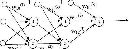
(3)(2)(3)(3)(2)(3)=ηδ1(3)xout?w=ηδ?w10=ηδ1(3),?w11,1 , 121xout,2
(2)(1)(2)(2)(1)(2)=ηδ1(2)xout?w=ηδ?w10=ηδ1(2),?w11,1 , 121xout,2
(2)(1)(2)(2)(1)(2)=ηδ2(2)xout?w=ηδ?w20=ηδ2(2),?w21 , ,1222xout,2
(1)(1)(1)?w10=ηδ1(1),?w11=ηδ1(1)x1 , ?w12=ηδ1(1)x2
(1)(1)(1)?w20=ηδ2(1),?w21=ηδ2(1)x1 , ?w22=ηδ2(1)x2
Above wt update is for a single training pattern
(corresponding to a learning step).
After a learning step is finished, next training pattern is submitted and the learning step is repeated.
Until all the patterns in the training set have been exhausted ? One epoch
Example: Solve the XOR problem using the following network architecture:
v1(1)o1(1)v1(2)
o1(2)
o2(2)v1(3)
v2(1)o2(1)v2(2)
The input vector consists of 4 patterns,
x1 = [0 0]T, x2 = [1 0]T, x3 = [1 1]T, x4 = [0, 1]T;
which corresponds to the desired vector of: d = [0, 1, 0, 1]T;
For randomly initialized weights and a learning rate of 0.8, the learning stops when the sum-squared err is less than 0.001 or the number of epochs reaches 2000. The
convergence is shown in the figure below.
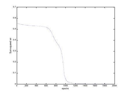
In this case, the output obtained is given as: y = [0.0219, 0.9769, 0.0239, 0.9768]T
After training, the weight matrix of each layer (1, 2, 3) is as follows,
bias
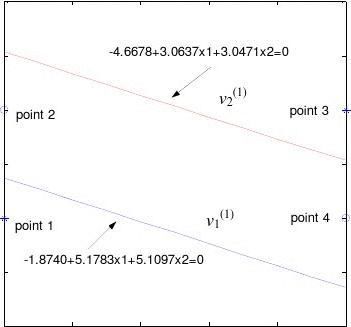
??1.875.175.10? w(1) =????4.663.063.04?
bias
??1.063.69?5.29?w(2) =? ??2.53?4.673.54?
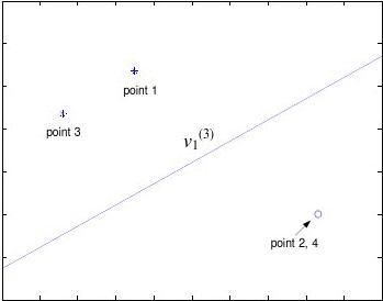
bias (3)w = [-0.36, 6.49, -6.5147]
Therefore the decision lines for the first hidden layer are:
-1.87 + 5.17·x1 + 5.10·x2 = 0 and -4.66 + 3.06·x1 + 3.04·x2 = 0.
x2
x1
The decision lines for the second hidden layer are:
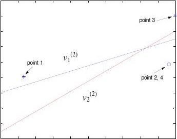
o2(1) o12
And the decision line for the output layer is:
o1o1(1)1
o2o22(2)
*********************
Source codes in Matlab
*********************
clear all;
close all;
X=[0 1 1 0;0 0 1 1]; o1o2(2)1
X=[ones(1,4);X];
d=[0 1 0 1];
H1=2;H2=2;
No=1;
W1=2*(rand(H1,3)-rand(H1,3));
W2=2*(rand(H2,H1+1)-rand(H2,H1+1)); W3=2*(rand(No,H2+1)-rand(No,H2+1)); err=1;
epoch=1;
yit=0.96;
while (err>0.001) & (epoch<2000)
err=0;
for iter=1:4
%% begin forward process
for i=1:H1
V1(i)=W1(i,:)*X(:,iter);
O1(i)=logsig(V1(i));
end
for i=1:H2
V2(i)=W2(i,:)*[1;O1'];
O2(i)=logsig(V2(i));
end
%%output layer
for i=1:No
V3(i)=W3(i,:)*[1;O2'];
Y(i,iter)=logsig(V3(i));
end
%%end forward process
%% begin backward pass
for i=1:No
De3(i)=(d(iter)-Y(i,iter))*Y(i,iter)*(1-Y(i,iter)); end
for i=1:H2
De2(i)=O2(i)*(1-O2(i))*W3(:,i+1)*De3; end
for i=1:H1
De1(i)=O1(i)*(1-O1(i))*(De2*W2(:,i+1)); end
%% end backward pass
%% weights update
W3=W3+yit*De3*[1;O2']'; for i=1:H2
W2(i,:)=W2(i,:)+yit*De2(i)*[1;O1']'; end
for i=1:H1
W1(i,:)=W1(i,:)+yit*De1(i)*X(:,iter)'; end
err=err+0.5*(d(iter)-Y(iter))^2; end %% end of one epoch Err(epoch)=err;
epoch=epoch+1;
end
Y
plot(Err)