图像处理课程设计报告(小初)
设计题目:
专业班级:通信08-02班
学生姓名: 吴丽霞
(以上小二号、行距40磅)
(A4纸打印)
题 目(三号,黑体,居中)
摘要(四号,黑体,居中)
图像中的噪声会妨碍人们对图像的理解,而图像去噪的目的就是去除图像中的噪声,提高人们对图像的认识程度,以便对图像作进一步地处理。该次课设就是用几种方法对图像的噪声进行处理,使图像增强。
1、均值滤波
均值滤波是在空间域对图象进行平滑处理的一种方法,易于实现,效果也挺好。
设噪声η(m,n)是加性噪声,其均值为0,方差(噪声功率)为σ2,而且噪声与图象f(m,n)不相关。
除了对噪声有上述假定之外,该算法还基于这样一种假设:图象是由许多灰度值相近的小块组成。这个假设大体上反映了许多图象的结构特征。(2)式表达的算法是由某像素领域内各点灰度值的平均值来代替该像素原来的灰度值。
可用模块反映领域平均算法的特征。对模版沿水平和垂直两个方向逐点移动,相当于用这样一个模块与图像进行卷积运算,从而平滑了整幅图象。模版内各系数和为1,用这样的模版处理常数图象时,图像没有变化;对一般图象处理后,整幅图像灰度的平均值可不变。
2、中值滤波
中值滤波是一种非线性处理技术,能抑制图象中的噪声。它是基于图象的这样一种特性:噪声往往以孤立的点的形式出现,这些点对应的象素很少,而图象则是由像素数较多、面积较大的小块构成。
在一维的情况下,中值滤波器是一个含有奇数个像素的窗口。在处理之后,位于窗口正中的像素的灰度值,用窗口内各像素灰度值的中值代替。例如若窗口长度为5,窗口中像素的灰度值为80、90、200、110、120,则中值为110,因为按小到大(或大到小)排序后,第三位的值是110。于是原理的窗口正中的灰度值200就由110取代。如果200是一个噪声的尖峰,则将被滤除。然而,如果它是一个信号,则滤波后就被消除,降低了分辨率。因此中值滤波在某些情况下抑制噪声,而在另一些情况下却会抑制信号。
中值滤波很容易推广到二维的情况。二维窗口的形式可以是正方形、近似圆形的或十字形的。在图像增强的具体应用中,中值滤波只能是一种抑制噪声的特殊工具,在处理中应监视其效果,以决定最终是福才有这种方案。实施过程中的关键问题是探讨一些快速算法。
3、低通滤波(Low-pass filter) 是一种过滤方式,规则为低频信号能正常通过,而超过设定临界值的高频信号则被阻隔、减弱。但是阻隔、减弱的幅度则会依据不同的频率以及不同的滤波程序(目的)而改变。它有的时候也被叫做高频去除过滤(high-cut filter)或者最高去除过滤(treble-cut filter)。低通过滤是高通过滤的对立。
(摘要正文小四,宋体,行距1.5倍)
Abstract
(英文摘要正文Times New Roman,小四,行距1.5倍)
1、 mean filter
The mean filter is in spatial domain smoothing of the image of a kind of method, easy to be realized, the effect is good too.
A noise η (m, n) is additive noise, the mean is 0, the variance (noise) for sigma 2, power and noise and image f (m, n) not related.
In addition to the noise outside the assumption, the algorithm is based on the assumption that the image is composed of many similar grey value of small pieces. The hypothesis that generally reflect many features of the structure of the image. (2) the algorithm of expression is a pixel field by each point in the average of the grey value to replace the pixels of the original grayscale value.
Can reflect the average algorithm modules field characteristics. For template along the vertical and horizontal directions to point mobile, equivalent to use so a module and image, and smooth operation convolution the image. Within the template coefficient and to 1, the use of such template image processing, image not constant changes; On the general image processing, the whole image can be unchanged.
2、 median filtering
The median filter is a nonlinear processing technology, can restrain the noise of the image. It is based on image such a feature: noise often in an isolated point, these points in the form of the corresponding pixel image is very few, and by the numbers of pixels the large area small pieces to form.
In one dimension, the median filter is a contains an odd number of pixels window. In the processing, is located in the window after is the pixel gray value, use within the window pixel values of the median instead. For example if the window for 5, the window the length of the pixel grayscale value for 80, 90, 200, 110, 120, the median for 110, according to the small to large because (or big to small), after the third order value is 110. So is the window of the principle of grey value by 110 instead of 200. If 200 is a noise, it will be the heights of filter. However, if it is a signal, the filter is eliminated after, and to reduce the resolution. So the median filter in some cases the noise elimination, and in some cases but will restrain signal.
The median filter is easy to spread to the 2 d. 2 d window form can be is a square, approximate circle or the cross. In image enhancement of the specific application, the median filter can reduce the noise is a kind of special tools, in dealing with the effect should be monitoring, with decision is ultimately blessing to just have this kind of plan. The key problems in the process of implementation is to explore some algorithms.
3、Low pass filtering (Low-pass the filter) is a kind of filtration method for Low frequency signal can be normal rules by, and more than the high frequency signal is critical value set was cut, abate. But cut off, abate range will according to different frequency and different filter program (purpose) and change. It sometimes also called high frequency remove filtering (high-how the filter) or the highest removal filter (treble-how the filter). Low through the filter high-pass filter is of the conflict.
目 录
一、设计目的、任务与要求
二、总体方案设计
三、各功能模块的主要实现程序
四、测试和调试
五、结论与心得
六、参考文献
一、设计目的、任务与要求(大标题均为四号,黑体)
(小标题为小四号,黑体;正文为小四号,宋体;单倍行距)
1、结合实例学习如何在视频显示程序中增加图像处理算法;
2、理解和掌握图像的线性变换和直方图均衡化的原理和应用;
3、了解平滑处理的算法和用途,学习使用均值滤波、中值滤波和拉普拉斯锐化进行图像增强处理的程序设计方法;
4、了解噪声模型及对图像添加噪声的基本方法;
5、了解图像变换的意义和手段;
6、熟悉傅里叶变换的基本性质;
7、热练掌握FFT方法及应用;
8、通过实验了解二维频谱的分布特点;
9、通过本实验掌握利用MATLAB编程实现数字图像的傅立叶变换及滤波
锐化和复原处理;
10、了解理想、巴特沃兹、高斯等不同滤波器的结构及滤波效果。
二、总体方案设计
自选黑白图像,用加噪声的方法获得有噪图像。
1、用图像平均的方法消除噪声并计算信噪比的改善。
2、用平滑滤波方法消除噪声并计算信噪比的改善。
3、用中值滤波方法消除噪声并计算信噪比的改善。
4、用理想低通滤波方法消除噪声并计算信噪比的改善。
5、用巴特沃斯低通滤波方法消除噪声并计算信噪比的改善。
更换不同图像及噪声重复以上滤波方法,观察并分析这些算法的应用场合。
(根据课程设计的具体情况,描述系统的具体构架,包括:功能模块的划分、系统运行的环境、选用的工具及主要实现功能的原理,系统总体架构可用方框图表示。)
三、各功能模块的主要实现程序
I=imread(‘原图像名.gif’); %读入原图像文件
imshow(I); %显示原图像
fftI=fft2(I); %二维离散傅立叶变换
sfftI=fftshift(fftI); %直流分量移到频谱中心
RR=real(sfftI); %取傅立叶变换的实部
f=fft2(J); %傅里叶变化
g=ifftshift(g); %傅里叶反变换
II=imag(sfftI); %取傅立叶变换的虚部
A=sqrt(RR.^2+II.^2); %计算频谱幅值
J=imnoise(I,'salt & pepper',0.02); %在原图上添加椒盐噪声
k=filter2(fspecial('average',A),J); %进行A×A模板平滑滤波
k=filter2(fspecial('average',A),J); %进行A×A模板平滑滤波
A=(A-min(min(A)))/(max(max(A))-min(min(A)))*225; %归一化
figure; %设定窗口
imshow(A); %显示原图像的频谱
snr=10*log(B/A) %计算信噪比
(主要的功能实现和函数要进行详细的说明,包括其用法,使用范围,及参数等)。
四、测试和调试
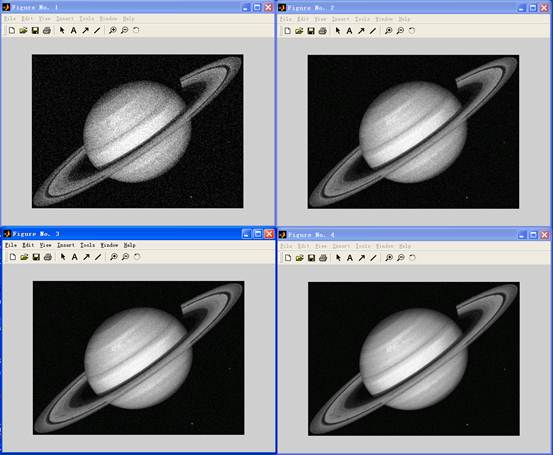
4图像平均法
例4.9
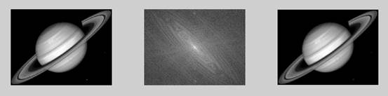
I=imread('saturn.tif'); %装入MATBLE图像是saturn
[M,N]=size(I); %建立矩阵
II1=zeros(M,N);
for i=1:16 %循环从1到16
II(:,:,i)=imnoise(I,'gaussian',0,0.01); %在原图I上,添加高斯噪声
II1=II1+double(II(:,:,i));
if or(or(i == 1,i == 4 ),or(i == 8,i ==16));
figure;
imshow(uint8(II1/i)); %分别以II1/1,II1/4,II1/8和II1/16命名四幅图
end
end
J1=double(II1)-double(I); %纯噪声
A=(std2(J1))^2; %噪声的方差
B=(std2(double(II1)))^2; %添加1幅同类图像后所得到的恢复图像的方差
snr1=10*log(B/A) %计算信噪比
J2=double(II1/4)-double(I);
C=(std2(II1/4))^2;
D=(std2(double(J2)))^2; %将4幅图像的均值添加在原图上所得到的恢复图像的方差
snr2=10*log(C/D)
J3=double(II1/8)-double(I);
E=(std2(double(II1/8)))^2; %将8幅图像的均值添加在原图上所得到的恢复图像的方差
F=(std2(J3))^2;
snr3=10*log(E/F)
J4=double(II1/16)-double(I);
H=(std2(double(II1/16)))^2; %将16幅图像的均值添加在原图上所得到的恢复图像的方差
G=(std2(J4))^2;
snr4=10*log(H/G)
结果:
snr1 = 1.3720
snr2 =6.1570
snr3 =15.0462
snr4 =45.5555
例4.10
I=imread('saturn.tif'); %装入MATBLE图像saturn
J=imnoise(I,'salt & pepper',0.02); %在原图上添加椒盐噪声,产生新的图像J
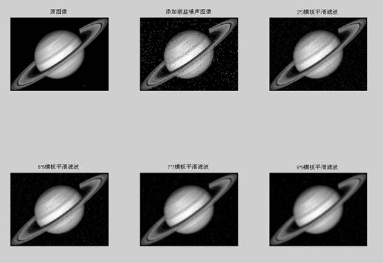
subplot(231),imshow(I);title('原图像'); %在2行3列的第1个位置,显示原图I,加标题
subplot(232),imshow(J);title('添加椒盐噪声图像'); % 在2行3列的第2个位置,显示添加噪声的图像J,加标题
k1=filter2(fspecial('average',3),J); %进行3×3模板平滑滤波
k2=filter2(fspecial('average',5),J); %进行5×5模板平滑滤波
k3=filter2(fspecial('average',7),J); %进行7×7模板平滑滤波
k4=filter2(fspecial('average',9),J); %进行9×9模板平滑滤波
subplot(233),imshow(uint8(k1));title('3*3模板平滑滤波'); %图像所在位置及名称
subplot(234),imshow(uint8(k2));title('5*5模板平滑滤波');
subplot(235),imshow(uint8(k3));title('7*7模板平滑滤波');
subplot(236),imshow(uint8(k4));title('9*9模板平滑滤波')
I2=double(J)-double(I) %纯噪声
A=(std2(I2/255))^2 %纯噪声的方差
B=std2(double(k1)/255)^2 %进行3×3模板平滑滤波后图像k1的方差
C=std2(double(k2)/255)^2 % 进行5×5模板平滑滤波后图像k2的方差
D=std2(double(k3)/255)^2 % 进行7×7模板平滑滤波后图像k3的方差
E=std2(double(k4)/255)^2 % 进行9×9模板平滑滤波后图像k4的方差
snr1=10*log(B/A) %计算信噪比
snr2=10*log(C/A)
snr3=10*log(D/A)
snr4=10*log(E/A)
所得结果:
snr1 =21.5874
snr2 =21.4311
snr3 =21.3249
snr4 = 21.2262
例4.11
I=imread(' saturn.tif'); %装入MATBLE图像saturn
J=imnoise(I,'salt & pepper',0.02); %在原图上添加椒盐噪声,产生新的图像J
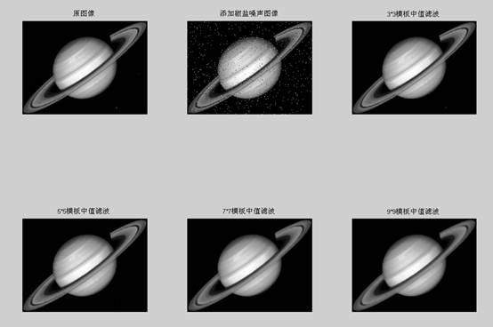
subplot(231),imshow(I);title('原图像'); %在2行3列的第1个位置,显示原图I,加标题
subplot(232),imshow(J);title('添加椒盐噪声图像'); % 在2行3列的第2个位置,显示添加噪声的图像J,加标题
k1=medfilt2(J); %进行3×3模板中值滤波
k2=medfilt2(J,[5 5]); %进行5×5模板中值滤波
k3=medfilt2(J,[7 7]); %进行7×7模板中值滤波
k4=medfilt2(J,[9 9]); %进行9×9模板中值滤波
subplot(233),imshow(k1);title('3*3模板中值滤波') %图像所在位置及名称
subplot(234),imshow(k2);title('5*5模板中值滤波')
subplot(235),imshow(k3);title('7*7模板中值滤波')
subplot(236),imshow(k4);title('9*9模板中值滤波')
I2=double(J)-double(I) %纯噪声
A=(std2(I2/255))^2 %纯噪声的方差
B=std2(double(k1)/255)^2 %进行3×3模板平滑滤波后图像k1的方差
C=std2(double(k2)/255)^2 %进行5×5模板平滑滤波后图像k2的方差
D=std2(double(k3)/255)^2 %进行7×7模板平滑滤波后图像k3的方差
E=std2(double(k4)/255)^2 %进行9×9模板平滑滤波后图像k4的方差
snr1=10*log(B/A) %计算信噪比
snr2=10*log(C/A)
snr3=10*log(D/A)
snr4=10*log(E/A)
结果:
snr1 =22.5069
snr2 =22.4962
snr3 =22.4869
snr4 = 22.4728
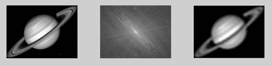
例4.13
J=imread('saturn.tif'); %装入MATBLE图像saturn
subplot(331);imshow(J);
J=double(J); %双精度变化
f=fft2(J); %傅里叶变化
g=fftshift(f); %数据矩阵平衡
subplot(332);imshow(log(abs(g)),[]),color(jet(64)); %显示傅里叶变换谱
[M,N]=size(f);
n1=floor(M/2); %设置浮点数
n2=floor(N/2);
d0=5;
for i=1:M
for j=1:N
d=sqrt((i-n1)^2+(j-n2)^2);
if d<=d0
h=1;
else
h=0;
end
g(i,j)=h*g(i,j);
end
end
g=ifftshift(g); %傅里叶反变换
g=uint8(real(ifft2(g))); %单精度的实部
subplot(333);
imshow(g);
J1=double(g)-double(J); %纯噪声
A=(std2(J1))^2; %噪声的方差
B=(std2(double(g)))^2; %恢复图像的方差
snr1=10*log(B/A) %计算信噪比
d0=5,snr1 = 21.8943

d0=15,snr1 = 38.2288
d0=45,snr1 = 56.9751
d0=65,snr1 = 64.7662

例4.14
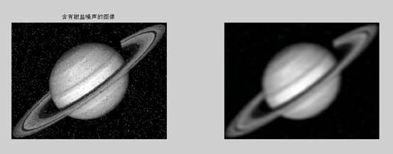
I=imread('saturn.tif'); %装入MATBLE图像saturn
J=imnoise(I,'salt & pepper',0.02); %在原图上添加椒盐噪声
subplot(121);imshow(J);
title('含有椒盐噪声的图像')
J=double(J); %进行双精度变换
f=fft2(J); %傅里叶变化
g=fftshift(f); %傅里叶反变化
[M,N]=size(f);
n=3;
d0=20; %设置初始值
n1=floor(M/2); %设置浮点数
n2=floor(N/2); % %建立矩阵
for i=1:M
for j=1:N
d=sqrt((i-n1)^2+(j-n2)^2);
h=1/(1+(d/d0)^(2*n));
g(i,j)=h*g(i,j);
end
end
I2=J-double(I); %纯噪声
g=ifftshift(g); %傅里叶反变化
G=uint8(real(ifft2(g))); %单精度实部
subplot(122);imshow(G);
A=std2(I2/255)^2
B=(std2(double(g)/255))^2
snr=10*log(B/A) %计算信噪比
结果:
A =0.0091
B =1.7048e+004
snr =144.4250
例4.9
I=imread('tire.tif');
[M,N]=size(I);
II1=zeros(M,N);
for i=1:16
II(:,:,i)=imnoise(I,'gaussian',0,0.01);
II1=II1+double(II(:,:,i));
if or(or(i == 1,i == 4 ),or(i == 8,i ==16));
figure;
imshow(uint8(II1/i));
end
end
J1=double(II1)-double(I);
A=(std2(J1))^2;
B=(std2(double(II1)))^2;
snr1=10*log(B/A)
J2=double(II1/4)-double(I);
C=(std2(II1/4))^2;
D=(std2(double(J2)))^2;
snr2=10*log(C/D)
J3=double(II1/8)-double(I);
E=(std2(double(II1/8)))^2;
F=(std2(J3))^2;
snr3=10*log(E/F)
J4=double(II1/16)-double(I);
H=(std2(double(II1/16)))^2;
G=(std2(J4))^2;
snr4=10*log(H/G)
snr1 =1.3455
snr2 = 6.0190
snr3 =14.5933
snr4 =44.0807

例4.10
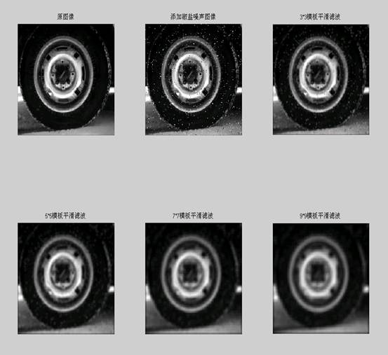
I=imread('tire.tif');
J=imnoise(I,'salt & pepper',0.02);
subplot(231),imshow(I);title('原图像');
subplot(232),imshow(J);title('添加椒盐噪声图像');
k1=filter2(fspecial('average',3),J);
k2=filter2(fspecial('average',5),J);
k3=filter2(fspecial('average',7),J);
k4=filter2(fspecial('average',9),J);
subplot(233),imshow(uint8(k1));title('3*3模板平滑滤波');
subplot(234),imshow(uint8(k2));title('5*5模板平滑滤波');
subplot(235),imshow(uint8(k3));title('7*7模板平滑滤波');
subplot(236),imshow(uint8(k4));title('9*9模板平滑滤波')
I2=double(J)-double(I)
A=(std2(I2/255))^2
B=std2(double(k1)/255)^2
C=std2(double(k2)/255)^2
D=std2(double(k3)/255)^2
E=std2(double(k4)/255)^2
snr1=10*log(B/A)
snr2=10*log(C/A)
snr3=10*log(D/A)
snr4=10*log(E/A)
snr1 = 18.8153
snr2 =17.9915
snr3 =17.1928
snr4 =16.3833
例4.11
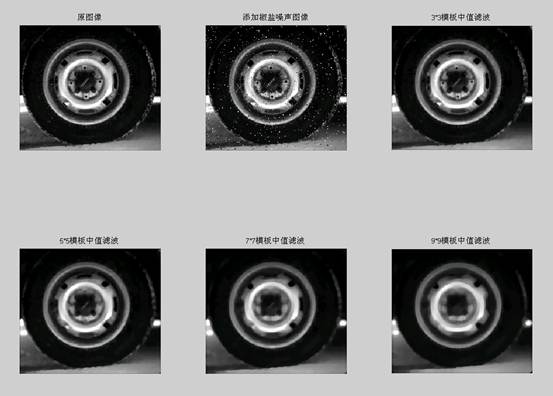
I=imread('tire.tif');
J=imnoise(I,'salt & pepper',0.02);
subplot(231),imshow(I);title('原图像');
subplot(232),imshow(J);title('添加椒盐噪声图像');
k1=medfilt2(J);
k2=medfilt2(J,[5 5]);
k3=medfilt2(J,[7 7]);
k4=medfilt2(J,[9 9]);
subplot(233),imshow(k1);title('3*3模板中值滤波')
subplot(234),imshow(k2);title('5*5模板中值滤波')
subplot(235),imshow(k3);title('7*7模板中值滤波')
subplot(236),imshow(k4);title('9*9模板中值滤波')
I2=double(J)-double(I)
A=(std2(I2/255))^2
B=std2(double(k1)/255)^2
C=std2(double(k2)/255)^2
D=std2(double(k3)/255)^2
E=std2(double(k4)/255)^2
snr1=10*log(B/A)
snr2=10*log(C/A)
snr3=10*log(D/A)
snr4=10*log(E/A)
A =0.0082
B = 0.0583
C = 0.0567
D =0.0547
E = 0.0517
snr1 =19.6435
snr2 =19.3577
snr3 =18.9948
snr4 = 18.4433
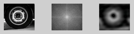
4.13
J=imread('tire.tif');
subplot(331);imshow(J);
J=double(J);
f=fft2(J);
g=fftshift(f);
subplot(332);imshow(log(abs(g)),[]),color(jet(64));
[M,N]=size(f);
n1=floor(M/2);
n2=floor(N/2);
d0=5;
for i=1:M
for j=1:N
d=sqrt((i-n1)^2+(j-n2)^2);
if d<=d0
h=1;
else
h=0;
end
g(i,j)=h*g(i,j);
end
end
g=ifftshift(g);
g=uint8(real(ifft2(g)));
subplot(333);
imshow(g);
J1=double(g)-double(J);
A=(std2(J1))^2;
B=(std2(double(g)))^2;
snr1=10*log(B/A)
d0=5, snr1 =0.0370
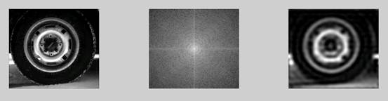
d0=15, snr1 =20.8364
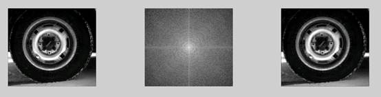
d0=45, snr1 =40.3386
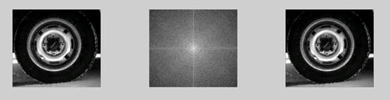
d0=65, snr1 =50.4833
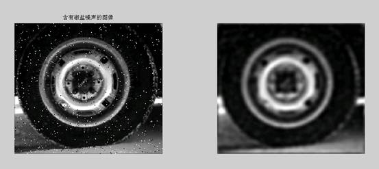
例4.14
I=imread('tire.tif');
J=imnoise(I,'salt & pepper',0.02);
subplot(121);imshow(J);
title('含有椒盐噪声的图像')
J=double(J);
f=fft2(J);
g=fftshift(f);
[M,N]=size(f);
n=3;
d0=20;
n1=floor(M/2);
n2=floor(N/2);
for i=1:M
for j=1:N
d=sqrt((i-n1)^2+(j-n2)^2);
h=1/(1+(d/d0)^(2*n));
g(i,j)=h*g(i,j);
end
end
I2=J-double(I);
g=ifftshift(g);
G=uint8(real(ifft2(g)));
subplot(122);imshow(G);
A=std2(I2/255)^2
B=(std2(double(g)/255))^2
snr=10*log(B/A)
结果:
A =0.0076
B =4.6718e+003
信噪比snr =133.2830
(按课程设计要求,选用多幅图像对程序进行测试,并提供系统的主要功能实现的效果图。并对调试中发现的问题做说明。)
五、结论与心得
1、比较例4.9各图,得出用图像平均的方法处理噪声时,进行平均的数量越多,噪声的影响就会越小,图像越来越清晰,故而信噪比会越来越高:snr1 = 1.3720 snr2 =6.1570 snr3 =15.0462 snr4 =45.5555 。
2、比较例4.10各图,得出用平滑滤波方法消除噪声时,所用模板尺寸增大时,对噪声的的消除有所增强,但同时所得的图像变得更加模糊,细节的锐化程度逐步减弱。信噪比越来越低:snr1 = 18.8153
snr2 =17.9915 snr3 =17.1928 snr4 =16.3833 。
3.、比较例4.11各图,得出用中值滤波方法消除噪声时,对过滤脉冲干燥及图像噪声非常有效。但也会使图像变得略有模糊,故而信噪比会略有减小:snr1 =19.6435 snr2 =19.3577 snr3 =18.9948 snr4 = 18.4433 。
对细节多(特别是点、线、尖顶)的图像不宜采用中值滤波法。
4、对应比较例4.10各图与例4.11各图,及他们各自的信噪比结果。得出添加椒盐噪声时,用中值滤波的方法处理噪声比用平滑滤波的方法处理噪声效果好。
5、比较例4.13各图,得出用理想低通滤波方法消除噪声,图像会由于截断半径不同而出现不同的效果。半径越大,噪声的处理效果越好,图像越来越清晰,信噪比会越来越高:
d0=5,snr = 21.8943;
d0=15, snr= 38.2288;
d0=45,snr= 56.9751;
d0=65,snr = 64.7662。
6、图像增强可分成两大类:频率域法和空间域法。前者把图像看成一种二维信号,对其进行基于二维傅里叶变换的信号增强。
7、采用低通滤波(即只让低频信号通过)法,可去掉图中的噪声;采用高通滤波法,则可增强边缘等高频信号,使模糊的图片变得清晰。具有代表性的空间域算法有局部求平均值法和中值滤波(取局部邻域中的中间像素值)法等,它们可用于去除或减弱噪声。
8、平滑一般用于消除图像噪声,但是也容易引起边缘的模糊。常用算法有均值滤波、中值滤波。锐化的目的在于突出物体的边缘轮廓,便于目标识别。
9、增强图象中的有用信息,它可以是一个失真的过程,其目的是要改善图像的视觉效果,针对给定图像的应用场合,有目的地强调图像的整体或局部特性,将原来不清晰的图像变得清晰或强调某些感兴趣的特征,扩大图像中不同物体特征之间的差别,抑制不感兴趣的特征,使之改善图像质量、丰富信息量,加强图像判读和识别效果,满足某些特殊分析的需要。
(设计过程中遇到的问题以及解决办法,有何心得体会)
六、参考文献
(写出具体的主要参考文献,标明其作者、出处、年代、若是期刊文章,还需要给出期刊名。网络的文章要给出网址。)
[1] 姚敏. 数字图像处理 .机械工业出版社 2007(五号,宋体,单倍行距)
[2] 陈怀琛 吴大正 高西全 MATLAB及电子信息课程中的应用. 电子工业出版社.2006
.