

20##-2014第1学期
计量经济学实验报告
实验(二):多元回归模型实验
学号: 姓名: 专业:
选课班级: 实验日期: 实验地点:
实验名称:多元回归模型实验
【实验目标、要求】
使学生掌握用Eviews做
1. 多元线性回归模型参数的OLS估计、统计检验、点预测和区间预测;
2. 非线性回归模型参数估计;
3. 受约束回归检验。
【实验内容】
用Eviews完成:
1. 多元线性回归模型参数的OLS估计、统计检验、点预测和区间预测;
2. 非线性回归模型的估计,并给出相应的结果。
3. 受约束回归检验。
实验内容以课后练习:以75页第8为例进行操作。
【实验步骤】
75页第8题
解:
(1)在Eviews中建立如下双对数变换模型:

估计结果如下:
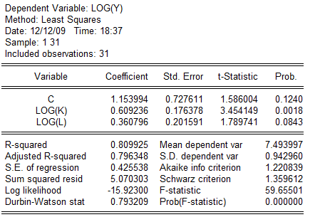
有上述数据可得,样本回归方程为:
t=(1.586) (3.454) (1.790)
分析:
1)拟合优度说明: 表明,lnY的79.6%的变化可以由lnK与lnL的变化来解释。当职工人数不变时,资产每增加1个单位,工业总产值将增加0.6092;当资产不变时,职工人数每增加1个单位,工业总产值将增加0.3068。
F统计量说明:若给定5%的显著性水平,临界值 =3.34,
 =2.048,由于F=59.66大于临界值,从总体上看,lnK与lnL对lnY的线性关系是显著的。
2)对参数的t值进行分析。lnK的参数所对应的t统计量3.454大于临界值的2.048,因此,该参数是显著的。但是lnL对应的t统计量1.790小于临界值2.048,该参数是不显著的。在假定的显著性水平为10%,临界值 =1.701,这时的参数就变为是显著的。
(2)由(1)可得, ,它表示资产投入K与劳动投入L的产出弹性近似为1,也就是说中国20##年的制造业总体呈现规模报酬不变的状态。下面用Eviews软件来进行检验。
1)原假设假定为 ,将原模型转化为
估计得到的结果为:
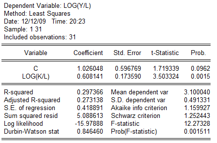
由上面数据可知,该方程F统计量值12.27大于临界值3.34,其参数也通过的检验。在无约束条件下方程的残差平方和为RSS1=5.0703,在约束条件下的方程残差平方和RSS2=5.0886,建立F统计量:

在5%的显著性水平下, =4.20,显然有F<,接受原假设,即可以认为中国20##年的制造业总体呈现规模报酬不变的状态。
第二篇:计量经济学实验八答案
1.

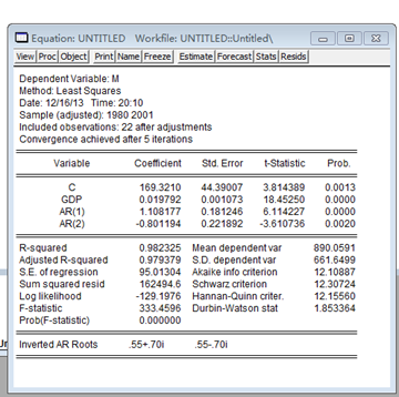
According to above table, we get the Durbin-Watson stat=0.627922 .
∵n=24 k=2,
Referring to the DW table ,we can get dl=1.27 du=1.45
∴there are first level positive relative between M and GDP
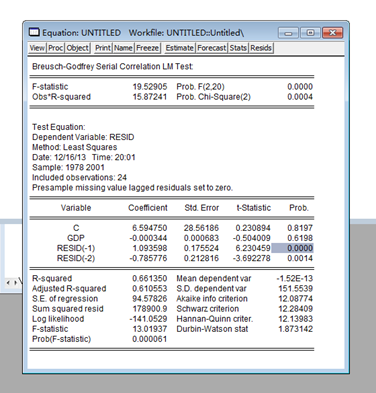
∵Obs*R-squared=15.8724>CHISQ(0.95,2)=5.991465
Besides t-statistic(resid(-1))= 6.230459>1.96besides t-Statistic(resid(-2))= -3.692278<-1.96
so there are second level relative between M and GDP
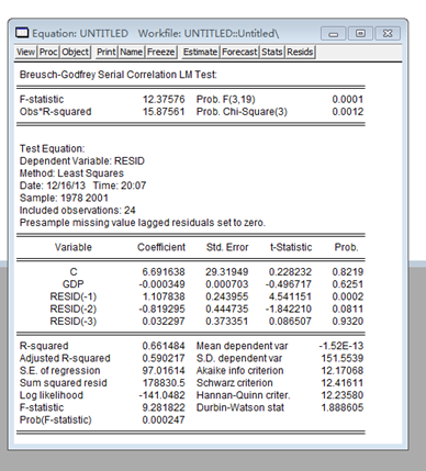
Because resid(-2) and resid(-3) are over 0.05, we can knowledge that here is not third-level positive
2.
3
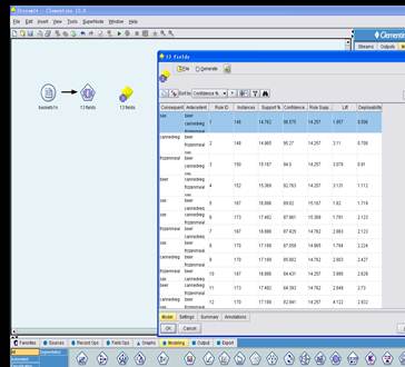
According to the picture we can conclude that the relationship between sex .cannedveg.frozenmeal and beer is tight
4.The following three equations were estimated using the 1,534 observations in 401K.RAW:

(1) Which of these three models do you prefer. Why?
I prefer to the second model. because ,the reasons is as following:
Comparing the above three equations, the second’s R-squard and Adjusted R-squard is maximum.
Referring to the rules of thumb,toetemp belongs to the total number, so it should use logarithmic functional form
all the t-Statistic of three Coefficient >1.96,so it is significant.
(2)Fill in the blanks in the estimation output for the second model.
