中南大学
模式识别与机器学习
实验报告
班 级 计科1203
学 号 0909121405
姓 名 雷亦恺
指导老师 梁毅雄
Programming Exercise 1: Linear Regression
Introduction
In this exercise, you will implement linear regression and get to see it work on data.
Before starting on this programming exercise, we strongly recommend watching the video lectures and completing the review questions for the associated topics.
To get started with the exercise, you will need to download the starter code and unzip its contents to the directory where you wish to complete the exercise.
If needed, use the cd command in Octave to change to this directory before starting this exercise.
You can also find instructions for installing Octave on the \Octave Installation" page on the course website.
Files included in this exercise
ex1.m - Octave script that will help step you through the exercise
ex1 multi.m - Octave script for the later parts of the exercise
ex1data1.txt - Dataset for linear regression with one variable
ex1data2.txt - Dataset for linear regression with multiple variables
submit.m - Submission script that sends your solutions to our servers
[*] warmUpExercise.m - Simple example function in Octave
[*] plotData.m - Function to display the dataset
[*] computeCost.m - Function to compute the cost of linear regression
[*] gradientDescent.m - Function to run gradient descent
[$] computeCostMulti.m - Cost function for multiple variables
[$] gradientDescentMulti.m - Gradient descent for multiple variables
[$] featureNormalize.m - Function to normalize features
[$] normalEqn.m - Function to compute the normal equations
* indicates les you will need to complete
$ indicates extra credit exercises
Throughout the exercise, you will be using the scripts ex1.m and ex1 multi.m.
These scripts set up the dataset for the problems and make calls to functions that you will write. You do not need to modify either of them.
You are only required to modify functions in other les, by following the instructions in this assignment.
For this programming exercise, you are only required to complete the rst part of the exercise to implement linear regression with one variable.
The second part of the exercise, which you may complete for extra credit, covers linear regression with multiple variables.
根据实验内容补全代码后如下:
(1)computeCost.m
function J = computeCost(X, y, theta)
%COMPUTECOST Compute cost for linear regression
% J = COMPUTECOST(X, y, theta) computes the cost of using theta as the
% parameter for linear regression to fit the data points in X and y
% Initialize some useful values
m = length(y); % number of training examples
% You need to return the following variables correctly
J = 0;
% ====================== YOUR CODE HERE ======================
% Instructions: Compute the cost of a particular choice of theta
% You should set J to the cost.
res = X*theta - y;
J = (res’ * res) / m*0.5;
% =========================================================================
end
(2)plotData.m
function plotData(x, y)
%PLOTDATA Plots the data points x and y into a new figure
% PLOTDATA(x,y) plots the data points and gives the figure axes labels of
% population and profit.
% ====================== YOUR CODE HERE ======================
% Instructions: Plot the training data into a figure using the
% "figure" and "plot" commands. Set the axes labels using
% the "xlabel" and "ylabel" commands. Assume the
% population and revenue data have been passed in
% as the x and y arguments of this function.
%
% Hint: You can use the 'rx' option with plot to have the markers
% appear as red crosses. Furthermore, you can make the
% markers larger by using plot(..., 'rx', 'MarkerSize', 10);
figure; % open a new figure window
plot(x,y,’rx’,’MarkerSize’,10);
xlabel(‘profit in $10,000s’);
ylabel(‘Population of City in 10,0000s’);
% ============================================================
end
(3)warmUpExercise.m
function A = warmUpExercise()
%WARMUPEXERCISE Example function in octave
% A = WARMUPEXERCISE() is an example function that returns the 5x5 identity matrix
A = [];
% ============= YOUR CODE HERE ==============
% Instructions: Return the 5x5 identity matrix
% In octave, we return values by defining which variables
% represent the return values (at the top of the file)
% and then set them accordingly.
A=eye(5);
% ===========================================
end
(4)featureNormalize.m
function [X_norm, mu, sigma] = featureNormalize(X)
%FEATURENORMALIZE Normalizes the features in X
% FEATURENORMALIZE(X) returns a normalized version of X where
% the mean value of each feature is 0 and the standard deviation
% is 1. This is often a good preprocessing step to do when
% working with learning algorithms.
% You need to set these values correctly
X_norm = X;
mu = zeros(1, size(X, 2));
sigma = zeros(1, size(X, 2));
% ====================== YOUR CODE HERE ======================
% Instructions: First, for each feature dimension, compute the mean
% of the feature and subtract it from the dataset,
% storing the mean value in mu. Next, compute the
% standard deviation of each feature and divide
% each feature by it's standard deviation, storing
% the standard deviation in sigma.
%
% Note that X is a matrix where each column is a
% feature and each row is an example. You need
% to perform the normalization separately for
% each feature.
%
% Hint: You might find the 'mean' and 'std' functions useful.
%
mu = mean(X_norm);
sigma = std(X_norm);
X_norm = (X_norm - repmat(mu, size(X,1), 1)) ./repmat(sigma , size(X, 1), 1);
% ============================================================
end
(5)computeCostMulti.m
function J = computeCostMulti(X, y, theta)
%COMPUTECOSTMULTI Compute cost for linear regression with multiple variables
% J = COMPUTECOSTMULTI(X, y, theta) computes the cost of using theta as the
% parameter for linear regression to fit the data points in X and y
% Initialize some useful values
m = length(y); % number of training examples
% You need to return the following variables correctly
J = 0;
% ====================== YOUR CODE HERE ======================
% Instructions: Compute the cost of a particular choice of theta
% You should set J to the cost.
res = X*theta - y;
J = (res’ * res ) /m *0.5;
% =========================================================================
End
(6)gradientDescent.m
function [theta, J_history] = gradientDescent(X, y, theta, alpha, num_iters)
%GRADIENTDESCENT Performs gradient descent to learn theta
% theta = GRADIENTDESENT(X, y, theta, alpha, num_iters) updates theta by
% taking num_iters gradient steps with learning rate alpha
% Initialize some useful values
m = length(y); % number of training examples
J_history = zeros(num_iters, 1);
for iter = 1:num_iters
% ====================== YOUR CODE HERE ======================
% Instructions: Perform a single gradient step on the parameter vector
% theta.
%
% Hint: While debugging, it can be useful to print out the values
% of the cost function (computeCost) and gradient here.
%
theta =theta - alpha / m *((X*theta - y))’* X)’;
% ============================================================
% Save the cost J in every iteration
J_history(iter) = computeCost(X, y, theta);
end
end
(7)gradientDescentMulti.m
function [theta, J_history] = gradientDescentMulti(X, y, theta, alpha, num_iters)
%GRADIENTDESCENTMULTI Performs gradient descent to learn theta
% theta = GRADIENTDESCENTMULTI(x, y, theta, alpha, num_iters) updates theta by
% taking num_iters gradient steps with learning rate alpha
% Initialize some useful values
m = length(y); % number of training examples
J_history = zeros(num_iters, 1);
for iter = 1:num_iters
% ====================== YOUR CODE HERE ======================
% Instructions: Perform a single gradient step on the parameter vector
% theta.
%
% Hint: While debugging, it can be useful to print out the values
% of the cost function (computeCostMulti) and gradient here.
%
t = ((X*theta - y)’ *X);
theta = theta - alpha /m * t;
% ============================================================
% Save the cost J in every iteration
J_history(iter) = computeCostMulti(X, y, theta);
end
end
(8)normalEqn.m
function [theta] = normalEqn(X, y)
%NORMALEQN Computes the closed-form solution to linear regression
% NORMALEQN(X,y) computes the closed-form solution to linear
% regression using the normal equations.
theta = zeros(size(X, 2), 1);
% ====================== YOUR CODE HERE ======================
% Instructions: Complete the code to compute the closed form solution
% to linear regression and put the result in theta.
%
theta = pinv(X’ *X)*X’ *y;
% ---------------------- Sample Solution ----------------------
% -------------------------------------------------------------
% ============================================================
end
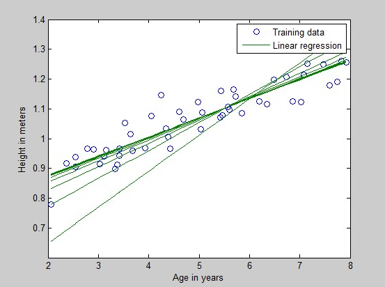
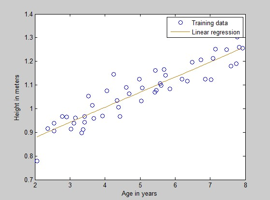
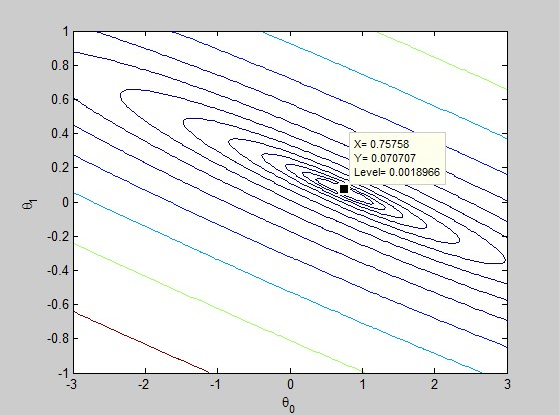
总体运行结果如图所示:

Programming Exercise 2: Logistic Regression
Introduction
In this exercise, you will implement logistic regression and apply it to two different datasets. Before starting on the programming exercise, we strongly recommend watching the video lectures and completing the review questions for the associated topics.
To get started with the exercise, you will need to download the starter code and unzip its contents to the directory where you wish to complete the exercise. If needed, use the cd command in Octave to change to this directory before starting this exercise.
You can also find instructions for installing Octave on the \Octave Installation" page on the course website.
Files included in this exercise
ex2.m - Octave script that will help step you through the exercise
ex2 reg.m - Octave script for the later parts of the exercise
ex2data1.txt - Training set for the rst half of the exercise
ex2data2.txt - Training set for the second half of the exercise
submitWeb.m - Alternative submission script
submit.m - Submission script that sends your solutions to our servers
mapFeature.m - Function to generate polynomial features
plotDecisionBounday.m - Function to plot classier's decision boundary
[*] plotData.m - Function to plot 2D classication data
[*] sigmoid.m - Sigmoid Function
[*] costFunction.m - Logistic Regression Cost Function
[*] predict.m - Logistic Regression Prediction Function
[*] costFunctionReg.m - Regularized Logistic Regression Cost
* indicates les you will need to complete
Throughout the exercise, you will be using the scripts ex2.m and ex2 reg.m.
These scripts set up the dataset for the problems and make calls to functions
that you will write. You do not need to modify either of them. You are only
required to modify functions in other les, by following the instructions in
this assignment.
根据实验内容补全代码后如下:
(1)plotData.m
function plotData(X, y)
%PLOTDATA Plots the data points X and y into a new figure
% PLOTDATA(x,y) plots the data points with + for the positive examples
% and o for the negative examples. X is assumed to be a Mx2 matrix.
% Create New Figure
figure; hold on;
% ====================== YOUR CODE HERE ======================
% Instructions: Plot the positive and negative examples on a
% 2D plot, using the option 'k+' for the positive
% examples and 'ko' for the negative examples.
%
positive = find (y == 1);
negative = find (y==0);
plot (X(positive, 1), X(positive,2), ‘k+’, ‘MarkerSize’, 7 ,’LineWidth’,2);
plot (X(negative, 1), X(negative,2), ‘ko’, ‘MarkerFaceColor’, ‘y’ ,’MarkSize’,7);
% =========================================================================
hold off;
end
(2)Sigmoid.m
function g = sigmoid(z)
%SIGMOID Compute sigmoid functoon
% J = SIGMOID(z) computes the sigmoid of z.
% You need to return the following variables correctly
g = zeros(size(z));
% ====================== YOUR CODE HERE ======================
% Instructions: Compute the sigmoid of each value of z (z can be a matrix,
% vector or scalar).
g = 1./(1+exp(-z));
% =============================================================
end
(3)costFunction.m
function [J, grad] = costFunction(theta, X, y)
%COSTFUNCTION Compute cost and gradient for logistic regression
% J = COSTFUNCTION(theta, X, y) computes the cost of using theta as the
% parameter for logistic regression and the gradient of the cost
% w.r.t. to the parameters.
% Initialize some useful values
m = length(y); % number of training examples
% You need to return the following variables correctly
J = 0;
grad = zeros(size(theta));
% ====================== YOUR CODE HERE ======================
% Instructions: Compute the cost of a particular choice of theta.
% You should set J to the cost.
% Compute the partial derivatives and set grad to the partial
% derivatives of the cost w.r.t. each parameter in theta
%
Hypothesis = sigmoid (X*theta);
J=1/m*sum(-y.*log(hypothesis)-(1-y).*log(1-hypothesis))+0.5*lambda/m*(theta(2:end)’*theta(2:end));
n = size(X,2);
grad(1) = 1/m*dot(hypothesis-y,X(:,1));
for i =2 : n
grad(i) = 1/m*dot(hypothesis - y,X(:,i))+lambda /m * theta(i);
% Note: grad should have the same dimensions as theta
%
% =============================================================
end
(4)Predict.m
function p = predict(theta, X)
%PREDICT Predict whether the label is 0 or 1 using learned logistic
%regression parameters theta
% p = PREDICT(theta, X) computes the predictions for X using a
% threshold at 0.5 (i.e., if sigmoid(theta'*x) >= 0.5, predict 1)
m = size(X, 1); % Number of training examples
% You need to return the following variables correctly
p = zeros(m, 1);
% ====================== YOUR CODE HERE ======================
% Instructions: Complete the following code to make predictions using
% your learned logistic regression parameters.
% You should set p to a vector of 0's and 1's
%
p= sigmoid(X*theta) >= 0.5;
% =========================================================================
end
(5)costFunctionReg.m
function [J, grad] = costFunctionReg(theta, X, y, lambda)
%COSTFUNCTIONREG Compute cost and gradient for logistic regression with regularization
% J = COSTFUNCTIONREG(theta, X, y, lambda) computes the cost of using
% theta as the parameter for regularized logistic regression and the
% gradient of the cost w.r.t. to the parameters.
% Initialize some useful values
m = length(y); % number of training examples
% You need to return the following variables correctly
J = 0;
grad = zeros(size(theta));
% ====================== YOUR CODE HERE ======================
% Instructions: Compute the cost of a particular choice of theta.
% You should set J to the cost.
% Compute the partial derivatives and set grad to the partial
% derivatives of the cost w.r.t. each parameter in theta
hypothesis = sigmoid (X*theta);
J=1/m*sum(-y.*log(hypothesis)-(1-y).*log(1-hypothesis))+0.5*lambda/m*(theta(2:end)’*theta(2:end));
n = size(X,2);
grad(1) = 1/m*dot(hypothesis-y,X(:,1));
for i =2 : n
grad(i) = 1/m*dot(hypothesis - y,X(:,i))+lambda /m * theta(i);
% =============================================================
End
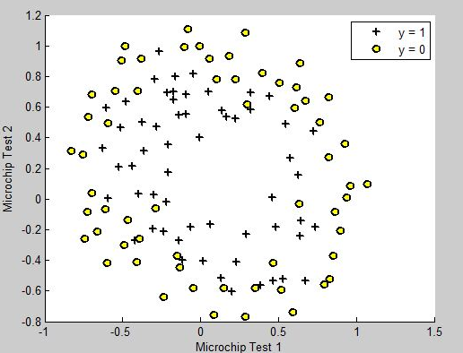
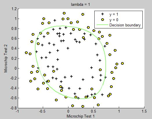
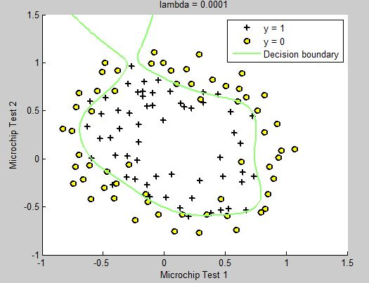
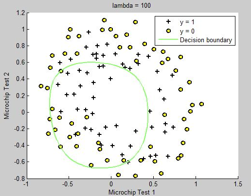
运行后结果如下: